Solution 5#
About#
So far, we have analysed satellite, model and ground-based observation data for one specific event.
Today, we would like to broaden our perspective and analyse more in detail the annual cycle and seasonality of dust and aerosols.
Tasks#
1. Brainstorm
What data, introduced to you in week 1, can be used for analysing the annual cylce and patterns of dust?
What aggregation level is required?
Which variables to analyse dust do you know and are available?
2. Download and plot monthly Metop-A/B/C GOME-2 Level 3 Absorbing Aerosol Index data for 2020
Download monthly Metop-A/B/C GOME-2 Absorbing Aerosol Index data for year 2020 and plot the monthly values as map featuring a geographical subset for bounding box N:70°, E:36°, S:0°, W:-50°
Hint
Some questions to reflect on
Can you identify some patterns? Describe the patterns you observe for each month.
Were some months more affected by desert dust than others in average?
3. Load AERONET observations and CAMS reanalysis (EAC4) time-series for Santa Cruz, Tenerife in 2020 and plot monthly aggregates in one plot
Load the time-series of daily aggregated AERONET observations and CAMS reanalysis (EAC4) for Santa Cruz, Tenerife in 2020, resample the values to monthly averages and plot the monthly averaged values together in one plot
Hint
Some questions to reflect on
Interpret the plotting result
Do the monthly patterns of AERONET observations and CAMS reanalysis look similar?
Do the patterns resemble those of Metop-A/B/C GOME-2 Level 3 Absorbing Aerosol Index data?
Load required libraries
import xarray as xr
import pandas as pd
from datetime import datetime

from IPython.display import HTML

import matplotlib.pyplot as plt
import matplotlib.colors
from matplotlib.cm import get_cmap
from matplotlib import animation
from matplotlib.axes import Axes

import cartopy.crs as ccrs
from cartopy.mpl.gridliner import LONGITUDE_FORMATTER, LATITUDE_FORMATTER
import cartopy.feature as cfeature
from cartopy.mpl.geoaxes import GeoAxes
GeoAxes._pcolormesh_patched = Axes.pcolormesh

import warnings
warnings.simplefilter(action = "ignore", category = RuntimeWarning)
Load helper functions
%run ../../functions.ipynb
1. Brainstorm#
The following data and variables can be used to analyse the annual cycle and patterns of dust:
-
Aerosol Optical Depth
Angstrom exponent
-
Absorbing Aerosol Index (AAI)
CAMS global reanalysis (EAC4)
Dust aerosol optical depth at 550 nm
2. Download and plot monthly Metop-A/B/C GOME-2 Level 3 Absorbing Aerosol Index data for year 2020#
The Metop-A/B/C GOME-3 Level 3 AAI data files can be downloaded from the TEMIS website in NetCDF data format. TEMIS offers the data of all three satellites Metop-A, -B and -C, which, combined, provide monthly measurements for the entire globe.
The following example uses monthly gridded AAI data from the three satellites Metop-A, -B, and -C for 2020.
Since the data is distributed in the NetCDF format, you can use the xarray function xr.open_mfdataset() to load the multiple netCDF files at once.
ds_a = xr.open_mfdataset('../../eodata/case_study/gome2/ESACCI-AEROSOL-L3-AAI-GOME2A-1M-2020*.nc',
                         concat_dim='time',
                         combine='nested')

aai_a=ds_a['absorbing_aerosol_index']
aai_a
<xarray.DataArray 'absorbing_aerosol_index' (time: 12, latitude: 180, longitude: 360)>
dask.array<concatenate, shape=(12, 180, 360), dtype=float32, chunksize=(1, 180, 360), chunktype=numpy.ndarray>
Coordinates:
  * longitude  (longitude) float32 -179.5 -178.5 -177.5 ... 177.5 178.5 179.5
  * latitude   (latitude) float32 -89.5 -88.5 -87.5 -86.5 ... 87.5 88.5 89.5
Dimensions without coordinates: time
Attributes:
    long_name:  Absorbing aerosol index averaged for each grid cell
units: 1- time: 12
- latitude: 180
- longitude: 360
- dask.array<chunksize=(1, 180, 360), meta=np.ndarray>
Array Chunk Bytes 2.97 MiB 253.12 kiB Shape (12, 180, 360) (1, 180, 360) Count 48 Tasks 12 Chunks Type float32 numpy.ndarray - longitude(longitude)float32-179.5 -178.5 ... 178.5 179.5
- long_name :
- Longitudes of the centre of the grid cells
- standard_name :
- longitude
- units :
- degrees
array([-179.5, -178.5, -177.5, ..., 177.5, 178.5, 179.5], dtype=float32)
- latitude(latitude)float32-89.5 -88.5 -87.5 ... 88.5 89.5
- long_name :
- Latitudes of the centre of the grid cells
- standard_name :
- latitude
- units :
- degrees
array([-89.5, -88.5, -87.5, -86.5, -85.5, -84.5, -83.5, -82.5, -81.5, -80.5,
       -79.5, -78.5, -77.5, -76.5, -75.5, -74.5, -73.5, -72.5, -71.5, -70.5,
       -69.5, -68.5, -67.5, -66.5, -65.5, -64.5, -63.5, -62.5, -61.5, -60.5,
       -59.5, -58.5, -57.5, -56.5, -55.5, -54.5, -53.5, -52.5, -51.5, -50.5,
       -49.5, -48.5, -47.5, -46.5, -45.5, -44.5, -43.5, -42.5, -41.5, -40.5,
       -39.5, -38.5, -37.5, -36.5, -35.5, -34.5, -33.5, -32.5, -31.5, -30.5,
       -29.5, -28.5, -27.5, -26.5, -25.5, -24.5, -23.5, -22.5, -21.5, -20.5,
       -19.5, -18.5, -17.5, -16.5, -15.5, -14.5, -13.5, -12.5, -11.5, -10.5,
        -9.5,  -8.5,  -7.5,  -6.5,  -5.5,  -4.5,  -3.5,  -2.5,  -1.5,  -0.5,
         0.5,   1.5,   2.5,   3.5,   4.5,   5.5,   6.5,   7.5,   8.5,   9.5,
        10.5,  11.5,  12.5,  13.5,  14.5,  15.5,  16.5,  17.5,  18.5,  19.5,
        20.5,  21.5,  22.5,  23.5,  24.5,  25.5,  26.5,  27.5,  28.5,  29.5,
        30.5,  31.5,  32.5,  33.5,  34.5,  35.5,  36.5,  37.5,  38.5,  39.5,
        40.5,  41.5,  42.5,  43.5,  44.5,  45.5,  46.5,  47.5,  48.5,  49.5,
        50.5,  51.5,  52.5,  53.5,  54.5,  55.5,  56.5,  57.5,  58.5,  59.5,
        60.5,  61.5,  62.5,  63.5,  64.5,  65.5,  66.5,  67.5,  68.5,  69.5,
        70.5,  71.5,  72.5,  73.5,  74.5,  75.5,  76.5,  77.5,  78.5,  79.5,
        80.5,  81.5,  82.5,  83.5,  84.5,  85.5,  86.5,  87.5,  88.5,  89.5],
      dtype=float32)
- long_name :
- Absorbing aerosol index averaged for each grid cell
- units :
- 1
The same process has to be repeated for the daily gridded AAI data from the satellites Metop-B and Metop-C respectively. Below, we load the GOME-2 Level 3 AAI data from the Metop-B satellite.
ds_b = xr.open_mfdataset('../../eodata/case_study/gome2/ESACCI-AEROSOL-L3-AAI-GOME2B-1M-2020*.nc',
                         concat_dim='time',
                         combine='nested')

aai_b =ds_b['absorbing_aerosol_index']
aai_b
<xarray.DataArray 'absorbing_aerosol_index' (time: 12, latitude: 180, longitude: 360)>
dask.array<concatenate, shape=(12, 180, 360), dtype=float32, chunksize=(1, 180, 360), chunktype=numpy.ndarray>
Coordinates:
  * longitude  (longitude) float32 -179.5 -178.5 -177.5 ... 177.5 178.5 179.5
  * latitude   (latitude) float32 -89.5 -88.5 -87.5 -86.5 ... 87.5 88.5 89.5
Dimensions without coordinates: time
Attributes:
    long_name:  Absorbing aerosol index averaged for each grid cell
units: 1- time: 12
- latitude: 180
- longitude: 360
- dask.array<chunksize=(1, 180, 360), meta=np.ndarray>
Array Chunk Bytes 2.97 MiB 253.12 kiB Shape (12, 180, 360) (1, 180, 360) Count 48 Tasks 12 Chunks Type float32 numpy.ndarray - longitude(longitude)float32-179.5 -178.5 ... 178.5 179.5
- long_name :
- Longitudes of the centre of the grid cells
- standard_name :
- longitude
- units :
- degrees
array([-179.5, -178.5, -177.5, ..., 177.5, 178.5, 179.5], dtype=float32)
- latitude(latitude)float32-89.5 -88.5 -87.5 ... 88.5 89.5
- long_name :
- Latitudes of the centre of the grid cells
- standard_name :
- latitude
- units :
- degrees
array([-89.5, -88.5, -87.5, -86.5, -85.5, -84.5, -83.5, -82.5, -81.5, -80.5,
       -79.5, -78.5, -77.5, -76.5, -75.5, -74.5, -73.5, -72.5, -71.5, -70.5,
       -69.5, -68.5, -67.5, -66.5, -65.5, -64.5, -63.5, -62.5, -61.5, -60.5,
       -59.5, -58.5, -57.5, -56.5, -55.5, -54.5, -53.5, -52.5, -51.5, -50.5,
       -49.5, -48.5, -47.5, -46.5, -45.5, -44.5, -43.5, -42.5, -41.5, -40.5,
       -39.5, -38.5, -37.5, -36.5, -35.5, -34.5, -33.5, -32.5, -31.5, -30.5,
       -29.5, -28.5, -27.5, -26.5, -25.5, -24.5, -23.5, -22.5, -21.5, -20.5,
       -19.5, -18.5, -17.5, -16.5, -15.5, -14.5, -13.5, -12.5, -11.5, -10.5,
        -9.5,  -8.5,  -7.5,  -6.5,  -5.5,  -4.5,  -3.5,  -2.5,  -1.5,  -0.5,
         0.5,   1.5,   2.5,   3.5,   4.5,   5.5,   6.5,   7.5,   8.5,   9.5,
        10.5,  11.5,  12.5,  13.5,  14.5,  15.5,  16.5,  17.5,  18.5,  19.5,
        20.5,  21.5,  22.5,  23.5,  24.5,  25.5,  26.5,  27.5,  28.5,  29.5,
        30.5,  31.5,  32.5,  33.5,  34.5,  35.5,  36.5,  37.5,  38.5,  39.5,
        40.5,  41.5,  42.5,  43.5,  44.5,  45.5,  46.5,  47.5,  48.5,  49.5,
        50.5,  51.5,  52.5,  53.5,  54.5,  55.5,  56.5,  57.5,  58.5,  59.5,
        60.5,  61.5,  62.5,  63.5,  64.5,  65.5,  66.5,  67.5,  68.5,  69.5,
        70.5,  71.5,  72.5,  73.5,  74.5,  75.5,  76.5,  77.5,  78.5,  79.5,
        80.5,  81.5,  82.5,  83.5,  84.5,  85.5,  86.5,  87.5,  88.5,  89.5],
      dtype=float32)
- long_name :
- Absorbing aerosol index averaged for each grid cell
- units :
- 1
And here, we load the daily gridded GOME-2 AAI Level 3 data files from the Metop-C satellite.
ds_c = xr.open_mfdataset('../../eodata/case_study/gome2/ESACCI-AEROSOL-L3-AAI-GOME2C-1M-2020*.nc',
                         concat_dim='time',
                         combine='nested')

aai_c=ds_c['absorbing_aerosol_index']
aai_c
<xarray.DataArray 'absorbing_aerosol_index' (time: 12, latitude: 180, longitude: 360)>
dask.array<concatenate, shape=(12, 180, 360), dtype=float32, chunksize=(1, 180, 360), chunktype=numpy.ndarray>
Coordinates:
  * longitude  (longitude) float32 -179.5 -178.5 -177.5 ... 177.5 178.5 179.5
  * latitude   (latitude) float32 -89.5 -88.5 -87.5 -86.5 ... 87.5 88.5 89.5
Dimensions without coordinates: time
Attributes:
    long_name:  Absorbing aerosol index averaged for each grid cell
units: 1- time: 12
- latitude: 180
- longitude: 360
- dask.array<chunksize=(1, 180, 360), meta=np.ndarray>
Array Chunk Bytes 2.97 MiB 253.12 kiB Shape (12, 180, 360) (1, 180, 360) Count 48 Tasks 12 Chunks Type float32 numpy.ndarray - longitude(longitude)float32-179.5 -178.5 ... 178.5 179.5
- long_name :
- Longitudes of the centre of the grid cells
- standard_name :
- longitude
- units :
- degrees
array([-179.5, -178.5, -177.5, ..., 177.5, 178.5, 179.5], dtype=float32)
- latitude(latitude)float32-89.5 -88.5 -87.5 ... 88.5 89.5
- long_name :
- Latitudes of the centre of the grid cells
- standard_name :
- latitude
- units :
- degrees
array([-89.5, -88.5, -87.5, -86.5, -85.5, -84.5, -83.5, -82.5, -81.5, -80.5,
       -79.5, -78.5, -77.5, -76.5, -75.5, -74.5, -73.5, -72.5, -71.5, -70.5,
       -69.5, -68.5, -67.5, -66.5, -65.5, -64.5, -63.5, -62.5, -61.5, -60.5,
       -59.5, -58.5, -57.5, -56.5, -55.5, -54.5, -53.5, -52.5, -51.5, -50.5,
       -49.5, -48.5, -47.5, -46.5, -45.5, -44.5, -43.5, -42.5, -41.5, -40.5,
       -39.5, -38.5, -37.5, -36.5, -35.5, -34.5, -33.5, -32.5, -31.5, -30.5,
       -29.5, -28.5, -27.5, -26.5, -25.5, -24.5, -23.5, -22.5, -21.5, -20.5,
       -19.5, -18.5, -17.5, -16.5, -15.5, -14.5, -13.5, -12.5, -11.5, -10.5,
        -9.5,  -8.5,  -7.5,  -6.5,  -5.5,  -4.5,  -3.5,  -2.5,  -1.5,  -0.5,
         0.5,   1.5,   2.5,   3.5,   4.5,   5.5,   6.5,   7.5,   8.5,   9.5,
        10.5,  11.5,  12.5,  13.5,  14.5,  15.5,  16.5,  17.5,  18.5,  19.5,
        20.5,  21.5,  22.5,  23.5,  24.5,  25.5,  26.5,  27.5,  28.5,  29.5,
        30.5,  31.5,  32.5,  33.5,  34.5,  35.5,  36.5,  37.5,  38.5,  39.5,
        40.5,  41.5,  42.5,  43.5,  44.5,  45.5,  46.5,  47.5,  48.5,  49.5,
        50.5,  51.5,  52.5,  53.5,  54.5,  55.5,  56.5,  57.5,  58.5,  59.5,
        60.5,  61.5,  62.5,  63.5,  64.5,  65.5,  66.5,  67.5,  68.5,  69.5,
        70.5,  71.5,  72.5,  73.5,  74.5,  75.5,  76.5,  77.5,  78.5,  79.5,
        80.5,  81.5,  82.5,  83.5,  84.5,  85.5,  86.5,  87.5,  88.5,  89.5],
      dtype=float32)
- long_name :
- Absorbing aerosol index averaged for each grid cell
- units :
- 1
Concatenate the data from the three satellites Metop-A, -B and -C
The next step is to concatenate the DataArrays from the three satellites Metop-A, -B and -C using a new dimension called satellite.
You can use the concat() function from the xarray library to do this. The result is a four-dimensional xarray.DataArray, with the dimensions satellite, time, latitude and longitude.
aai_concat = xr.concat([aai_a,aai_b,aai_c], dim='satellite')
aai_concat
<xarray.DataArray 'absorbing_aerosol_index' (satellite: 3, time: 12, latitude: 180, longitude: 360)>
dask.array<concatenate, shape=(3, 12, 180, 360), dtype=float32, chunksize=(1, 1, 180, 360), chunktype=numpy.ndarray>
Coordinates:
  * longitude  (longitude) float32 -179.5 -178.5 -177.5 ... 177.5 178.5 179.5
  * latitude   (latitude) float32 -89.5 -88.5 -87.5 -86.5 ... 87.5 88.5 89.5
Dimensions without coordinates: satellite, time
Attributes:
    long_name:  Absorbing aerosol index averaged for each grid cell
units: 1- satellite: 3
- time: 12
- latitude: 180
- longitude: 360
- dask.array<chunksize=(1, 1, 180, 360), meta=np.ndarray>
Array Chunk Bytes 8.90 MiB 253.12 kiB Shape (3, 12, 180, 360) (1, 1, 180, 360) Count 216 Tasks 36 Chunks Type float32 numpy.ndarray - longitude(longitude)float32-179.5 -178.5 ... 178.5 179.5
- long_name :
- Longitudes of the centre of the grid cells
- standard_name :
- longitude
- units :
- degrees
array([-179.5, -178.5, -177.5, ..., 177.5, 178.5, 179.5], dtype=float32)
- latitude(latitude)float32-89.5 -88.5 -87.5 ... 88.5 89.5
- long_name :
- Latitudes of the centre of the grid cells
- standard_name :
- latitude
- units :
- degrees
array([-89.5, -88.5, -87.5, -86.5, -85.5, -84.5, -83.5, -82.5, -81.5, -80.5,
       -79.5, -78.5, -77.5, -76.5, -75.5, -74.5, -73.5, -72.5, -71.5, -70.5,
       -69.5, -68.5, -67.5, -66.5, -65.5, -64.5, -63.5, -62.5, -61.5, -60.5,
       -59.5, -58.5, -57.5, -56.5, -55.5, -54.5, -53.5, -52.5, -51.5, -50.5,
       -49.5, -48.5, -47.5, -46.5, -45.5, -44.5, -43.5, -42.5, -41.5, -40.5,
       -39.5, -38.5, -37.5, -36.5, -35.5, -34.5, -33.5, -32.5, -31.5, -30.5,
       -29.5, -28.5, -27.5, -26.5, -25.5, -24.5, -23.5, -22.5, -21.5, -20.5,
       -19.5, -18.5, -17.5, -16.5, -15.5, -14.5, -13.5, -12.5, -11.5, -10.5,
        -9.5,  -8.5,  -7.5,  -6.5,  -5.5,  -4.5,  -3.5,  -2.5,  -1.5,  -0.5,
         0.5,   1.5,   2.5,   3.5,   4.5,   5.5,   6.5,   7.5,   8.5,   9.5,
        10.5,  11.5,  12.5,  13.5,  14.5,  15.5,  16.5,  17.5,  18.5,  19.5,
        20.5,  21.5,  22.5,  23.5,  24.5,  25.5,  26.5,  27.5,  28.5,  29.5,
        30.5,  31.5,  32.5,  33.5,  34.5,  35.5,  36.5,  37.5,  38.5,  39.5,
        40.5,  41.5,  42.5,  43.5,  44.5,  45.5,  46.5,  47.5,  48.5,  49.5,
        50.5,  51.5,  52.5,  53.5,  54.5,  55.5,  56.5,  57.5,  58.5,  59.5,
        60.5,  61.5,  62.5,  63.5,  64.5,  65.5,  66.5,  67.5,  68.5,  69.5,
        70.5,  71.5,  72.5,  73.5,  74.5,  75.5,  76.5,  77.5,  78.5,  79.5,
        80.5,  81.5,  82.5,  83.5,  84.5,  85.5,  86.5,  87.5,  88.5,  89.5],
      dtype=float32)
- long_name :
- Absorbing aerosol index averaged for each grid cell
- units :
- 1
Retrieve time coordinate information and assign time coordinates for the time dimension
You can see that the resulting xarray.DataArray holds coordinate information for the two spatial dimensions longitude and latitude, but not for time and satellite.
However, the coordinates for time will be important for plotting the data as we need to know which month the data is valid. Thus, a next step is to assign coordinates to the time dimension.
With the help of the Python library pandas, you can build a DateTime time series for the months in 2020, from 1 January to 31 December 2021.
time_coords = pd.date_range(datetime.strptime('01-2020','%m-%Y'), periods=12, freq='m').strftime("%Y-%m").astype('datetime64[ns]')
time_coords
DatetimeIndex(['2020-01-01', '2020-02-01', '2020-03-01', '2020-04-01',
               '2020-05-01', '2020-06-01', '2020-07-01', '2020-08-01',
               '2020-09-01', '2020-10-01', '2020-11-01', '2020-12-01'],
              dtype='datetime64[ns]', freq=None)
The final step is to assign the pandas time series object time_coords to the aai_concat DataArray object. You can use the assign_coords() function from xarray. The result is that the time coordinates have now been assigned values. The only dimension the remains unassigned is satellite.
aai_concat = aai_concat.assign_coords(time=time_coords)
aai_concat
<xarray.DataArray 'absorbing_aerosol_index' (satellite: 3, time: 12, latitude: 180, longitude: 360)>
dask.array<concatenate, shape=(3, 12, 180, 360), dtype=float32, chunksize=(1, 1, 180, 360), chunktype=numpy.ndarray>
Coordinates:
  * longitude  (longitude) float32 -179.5 -178.5 -177.5 ... 177.5 178.5 179.5
  * latitude   (latitude) float32 -89.5 -88.5 -87.5 -86.5 ... 87.5 88.5 89.5
  * time       (time) datetime64[ns] 2020-01-01 2020-02-01 ... 2020-12-01
Dimensions without coordinates: satellite
Attributes:
    long_name:  Absorbing aerosol index averaged for each grid cell
units: 1- satellite: 3
- time: 12
- latitude: 180
- longitude: 360
- dask.array<chunksize=(1, 1, 180, 360), meta=np.ndarray>
Array Chunk Bytes 8.90 MiB 253.12 kiB Shape (3, 12, 180, 360) (1, 1, 180, 360) Count 216 Tasks 36 Chunks Type float32 numpy.ndarray - longitude(longitude)float32-179.5 -178.5 ... 178.5 179.5
- long_name :
- Longitudes of the centre of the grid cells
- standard_name :
- longitude
- units :
- degrees
array([-179.5, -178.5, -177.5, ..., 177.5, 178.5, 179.5], dtype=float32)
- latitude(latitude)float32-89.5 -88.5 -87.5 ... 88.5 89.5
- long_name :
- Latitudes of the centre of the grid cells
- standard_name :
- latitude
- units :
- degrees
array([-89.5, -88.5, -87.5, -86.5, -85.5, -84.5, -83.5, -82.5, -81.5, -80.5, -79.5, -78.5, -77.5, -76.5, -75.5, -74.5, -73.5, -72.5, -71.5, -70.5, -69.5, -68.5, -67.5, -66.5, -65.5, -64.5, -63.5, -62.5, -61.5, -60.5, -59.5, -58.5, -57.5, -56.5, -55.5, -54.5, -53.5, -52.5, -51.5, -50.5, -49.5, -48.5, -47.5, -46.5, -45.5, -44.5, -43.5, -42.5, -41.5, -40.5, -39.5, -38.5, -37.5, -36.5, -35.5, -34.5, -33.5, -32.5, -31.5, -30.5, -29.5, -28.5, -27.5, -26.5, -25.5, -24.5, -23.5, -22.5, -21.5, -20.5, -19.5, -18.5, -17.5, -16.5, -15.5, -14.5, -13.5, -12.5, -11.5, -10.5, -9.5, -8.5, -7.5, -6.5, -5.5, -4.5, -3.5, -2.5, -1.5, -0.5, 0.5, 1.5, 2.5, 3.5, 4.5, 5.5, 6.5, 7.5, 8.5, 9.5, 10.5, 11.5, 12.5, 13.5, 14.5, 15.5, 16.5, 17.5, 18.5, 19.5, 20.5, 21.5, 22.5, 23.5, 24.5, 25.5, 26.5, 27.5, 28.5, 29.5, 30.5, 31.5, 32.5, 33.5, 34.5, 35.5, 36.5, 37.5, 38.5, 39.5, 40.5, 41.5, 42.5, 43.5, 44.5, 45.5, 46.5, 47.5, 48.5, 49.5, 50.5, 51.5, 52.5, 53.5, 54.5, 55.5, 56.5, 57.5, 58.5, 59.5, 60.5, 61.5, 62.5, 63.5, 64.5, 65.5, 66.5, 67.5, 68.5, 69.5, 70.5, 71.5, 72.5, 73.5, 74.5, 75.5, 76.5, 77.5, 78.5, 79.5, 80.5, 81.5, 82.5, 83.5, 84.5, 85.5, 86.5, 87.5, 88.5, 89.5], dtype=float32) - time(time)datetime64[ns]2020-01-01 ... 2020-12-01
array(['2020-01-01T00:00:00.000000000', '2020-02-01T00:00:00.000000000',
       '2020-03-01T00:00:00.000000000', '2020-04-01T00:00:00.000000000',
       '2020-05-01T00:00:00.000000000', '2020-06-01T00:00:00.000000000',
       '2020-07-01T00:00:00.000000000', '2020-08-01T00:00:00.000000000',
       '2020-09-01T00:00:00.000000000', '2020-10-01T00:00:00.000000000',
       '2020-11-01T00:00:00.000000000', '2020-12-01T00:00:00.000000000'],
      dtype='datetime64[ns]')
- long_name :
- Absorbing aerosol index averaged for each grid cell
- units :
- 1
Combine AAI data from the three satellites Metop-A, -B and -C onto one single grid
Since the final aim is to combine the data from the three satellites Metop-A, -B and -C onto one single grid, the next step is to reduce the satellite dimension. You can do this by applying the reduce function mean to the aai_concat Data Array. The dimension (dim) to be reduced is the satellite dimension.
This function builds the average of all data points within a grid cell. The resulting xarray.DataArray has three dimensions time, latitude and longitude.
aai_combined = aai_concat.mean(dim='satellite')
aai_combined
<xarray.DataArray 'absorbing_aerosol_index' (time: 12, latitude: 180, longitude: 360)>
dask.array<mean_agg-aggregate, shape=(12, 180, 360), dtype=float32, chunksize=(1, 180, 360), chunktype=numpy.ndarray>
Coordinates:
  * longitude  (longitude) float32 -179.5 -178.5 -177.5 ... 177.5 178.5 179.5
  * latitude   (latitude) float32 -89.5 -88.5 -87.5 -86.5 ... 87.5 88.5 89.5
  * time       (time) datetime64[ns] 2020-01-01 2020-02-01 ... 2020-12-01
- time: 12
- latitude: 180
- longitude: 360
- dask.array<chunksize=(1, 180, 360), meta=np.ndarray>
Array Chunk Bytes 2.97 MiB 253.12 kiB Shape (12, 180, 360) (1, 180, 360) Count 264 Tasks 12 Chunks Type float32 numpy.ndarray - longitude(longitude)float32-179.5 -178.5 ... 178.5 179.5
- long_name :
- Longitudes of the centre of the grid cells
- standard_name :
- longitude
- units :
- degrees
array([-179.5, -178.5, -177.5, ..., 177.5, 178.5, 179.5], dtype=float32)
- latitude(latitude)float32-89.5 -88.5 -87.5 ... 88.5 89.5
- long_name :
- Latitudes of the centre of the grid cells
- standard_name :
- latitude
- units :
- degrees
array([-89.5, -88.5, -87.5, -86.5, -85.5, -84.5, -83.5, -82.5, -81.5, -80.5, -79.5, -78.5, -77.5, -76.5, -75.5, -74.5, -73.5, -72.5, -71.5, -70.5, -69.5, -68.5, -67.5, -66.5, -65.5, -64.5, -63.5, -62.5, -61.5, -60.5, -59.5, -58.5, -57.5, -56.5, -55.5, -54.5, -53.5, -52.5, -51.5, -50.5, -49.5, -48.5, -47.5, -46.5, -45.5, -44.5, -43.5, -42.5, -41.5, -40.5, -39.5, -38.5, -37.5, -36.5, -35.5, -34.5, -33.5, -32.5, -31.5, -30.5, -29.5, -28.5, -27.5, -26.5, -25.5, -24.5, -23.5, -22.5, -21.5, -20.5, -19.5, -18.5, -17.5, -16.5, -15.5, -14.5, -13.5, -12.5, -11.5, -10.5, -9.5, -8.5, -7.5, -6.5, -5.5, -4.5, -3.5, -2.5, -1.5, -0.5, 0.5, 1.5, 2.5, 3.5, 4.5, 5.5, 6.5, 7.5, 8.5, 9.5, 10.5, 11.5, 12.5, 13.5, 14.5, 15.5, 16.5, 17.5, 18.5, 19.5, 20.5, 21.5, 22.5, 23.5, 24.5, 25.5, 26.5, 27.5, 28.5, 29.5, 30.5, 31.5, 32.5, 33.5, 34.5, 35.5, 36.5, 37.5, 38.5, 39.5, 40.5, 41.5, 42.5, 43.5, 44.5, 45.5, 46.5, 47.5, 48.5, 49.5, 50.5, 51.5, 52.5, 53.5, 54.5, 55.5, 56.5, 57.5, 58.5, 59.5, 60.5, 61.5, 62.5, 63.5, 64.5, 65.5, 66.5, 67.5, 68.5, 69.5, 70.5, 71.5, 72.5, 73.5, 74.5, 75.5, 76.5, 77.5, 78.5, 79.5, 80.5, 81.5, 82.5, 83.5, 84.5, 85.5, 86.5, 87.5, 88.5, 89.5], dtype=float32) - time(time)datetime64[ns]2020-01-01 ... 2020-12-01
array(['2020-01-01T00:00:00.000000000', '2020-02-01T00:00:00.000000000',
       '2020-03-01T00:00:00.000000000', '2020-04-01T00:00:00.000000000',
       '2020-05-01T00:00:00.000000000', '2020-06-01T00:00:00.000000000',
       '2020-07-01T00:00:00.000000000', '2020-08-01T00:00:00.000000000',
       '2020-09-01T00:00:00.000000000', '2020-10-01T00:00:00.000000000',
       '2020-11-01T00:00:00.000000000', '2020-12-01T00:00:00.000000000'],
      dtype='datetime64[ns]')
Visualize AAI data with data from the three satellites Metop-A, -B and C combined on one single grid
The next step is to visualize the Absorbing Aerosol Index data for one time step. You can use the function visualize_pcolormesh for it.
You can use afmhot_r as color map, ccrs.PlateCarree() as projection and by applying dt.strftime('%Y-%m-%d').data to the time coordinate variable, you can add the valid time step to the title of the plot.
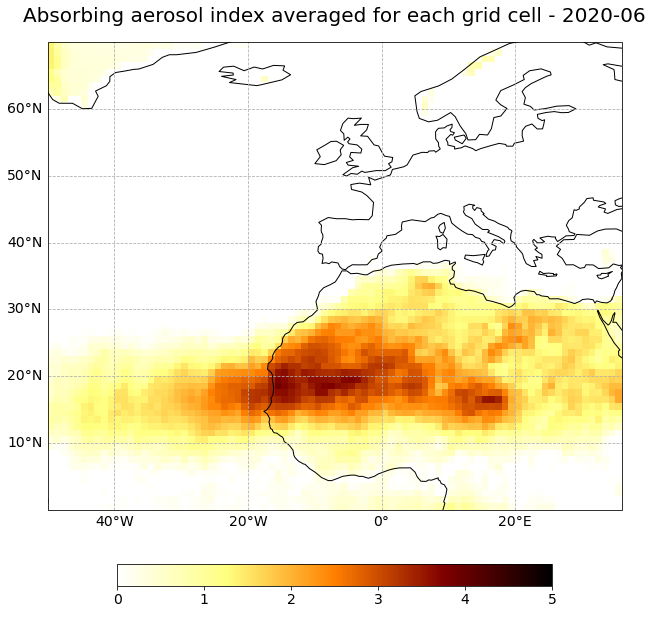
Let us plot a geographic subset over Western Africa and the Atlantic (N: 70, E:36, S:0, W:-50).
Plot different months. Can you identfy some patterns? Were some months more affected by desert dust than others in average?
month=5
visualize_pcolormesh(data_array=aai_combined[month,:,:],
                     longitude=aai_combined.longitude,
                     latitude=aai_combined.latitude,
                     projection=ccrs.PlateCarree(),
                     color_scale='afmhot_r',
                     unit=' ',
                     long_name=aai_a.long_name + ' - ' + str(aai_combined.time[month].dt.strftime('%Y-%m').data),
                     vmin=0,
                     vmax=5,
                     lonmin=-50,
                     lonmax=36,
                     latmin=0,
                     latmax=70.,
                     set_global=False)
(<Figure size 1440x720 with 2 Axes>,
 <GeoAxesSubplot:title={'center':'Absorbing aerosol index averaged for each grid cell - 2020-06'}>)
3. Load AERONET and CAMS reanalysis (EAC4) time-series for Santa Cruz, Tenerife in 2020 and plot monthly aggregates#
The file is a result from Day 2 - Assignment and the created pandas dataframe was saved as a csv file under ../eodata/case_study/2020_ts_cams_aeronet.csv. We can open it with the pandas function read_table(). We additonally set specific keyword arguments:
delimiter: specify the delimiter in the text file, e.g. comma
You see below that the resulting dataframe has 366 rows and 5 columns: time, longitude, latitude, duaod550, AOD_500nm. The columns duaod550 are the dust aersol optical depth values from the CAMS reanalysis and AOD_500nm are the station measurements from AERONET.
df = pd.read_csv('../../eodata/case_study/2020_ts_cams_aeronet.csv', delimiter=',')
df
| time | longitude | latitude | duaod550 | AOD_500nm | |
|---|---|---|---|---|---|
| 0 | 2020-01-01 | -16.25 | 28.25 | 0.062677 | 0.094487 |
| 1 | 2020-01-02 | -16.25 | 28.25 | 0.121897 | NaN |
| 2 | 2020-01-03 | -16.25 | 28.25 | 0.064505 | 0.075765 |
| 3 | 2020-01-04 | -16.25 | 28.25 | 0.006812 | 0.098110 |
| 4 | 2020-01-05 | -16.25 | 28.25 | 0.001114 | 0.085672 |
| ... | ... | ... | ... | ... | ... |
| 361 | 2020-12-27 | -16.25 | 28.25 | 0.069240 | 0.134366 |
| 362 | 2020-12-28 | -16.25 | 28.25 | 0.215455 | 0.415433 |
| 363 | 2020-12-29 | -16.25 | 28.25 | 0.182338 | 0.320463 |
| 364 | 2020-12-30 | -16.25 | 28.25 | 0.072843 | 0.095342 |
| 365 | 2020-12-31 | -16.25 | 28.25 | 0.010482 | 0.033297 |
366 rows × 5 columns
Let us now convert the time column to a DateTimeIndex format with the function to_datetime(). Important here, you have to specify the format of the index string: %Y-%m-%d.
df.index = pd.to_datetime(df.time, format = '%Y-%m-%d')
df
| time | longitude | latitude | duaod550 | AOD_500nm | |
|---|---|---|---|---|---|
| time | |||||
| 2020-01-01 | 2020-01-01 | -16.25 | 28.25 | 0.062677 | 0.094487 |
| 2020-01-02 | 2020-01-02 | -16.25 | 28.25 | 0.121897 | NaN |
| 2020-01-03 | 2020-01-03 | -16.25 | 28.25 | 0.064505 | 0.075765 |
| 2020-01-04 | 2020-01-04 | -16.25 | 28.25 | 0.006812 | 0.098110 |
| 2020-01-05 | 2020-01-05 | -16.25 | 28.25 | 0.001114 | 0.085672 |
| ... | ... | ... | ... | ... | ... |
| 2020-12-27 | 2020-12-27 | -16.25 | 28.25 | 0.069240 | 0.134366 |
| 2020-12-28 | 2020-12-28 | -16.25 | 28.25 | 0.215455 | 0.415433 |
| 2020-12-29 | 2020-12-29 | -16.25 | 28.25 | 0.182338 | 0.320463 |
| 2020-12-30 | 2020-12-30 | -16.25 | 28.25 | 0.072843 | 0.095342 |
| 2020-12-31 | 2020-12-31 | -16.25 | 28.25 | 0.010482 | 0.033297 |
366 rows × 5 columns
We are interested in the monthly averages of aerosol optical depth in 2020. With the function resample(), we can create the monthly averages based on the daily AOD values. The result is a data frame with 12 row entries and 4 columns.
df_resample = df.resample('1M').mean()
df_resample
| longitude | latitude | duaod550 | AOD_500nm | |
|---|---|---|---|---|
| time | ||||
| 2020-01-31 | -16.25 | 28.25 | 0.034638 | 0.117633 |
| 2020-02-29 | -16.25 | 28.25 | 0.163640 | 0.245622 |
| 2020-03-31 | -16.25 | 28.25 | 0.047373 | 0.133028 |
| 2020-04-30 | -16.25 | 28.25 | 0.002262 | 0.085046 |
| 2020-05-31 | -16.25 | 28.25 | 0.018629 | 0.099021 |
| 2020-06-30 | -16.25 | 28.25 | 0.147789 | 0.082430 |
| 2020-07-31 | -16.25 | 28.25 | 0.256171 | 0.357828 |
| 2020-08-31 | -16.25 | 28.25 | 0.149128 | 0.267296 |
| 2020-09-30 | -16.25 | 28.25 | 0.199188 | 0.195343 |
| 2020-10-31 | -16.25 | 28.25 | 0.076314 | 0.138351 |
| 2020-11-30 | -16.25 | 28.25 | 0.038752 | 0.106877 |
| 2020-12-31 | -16.25 | 28.25 | 0.044603 | 0.096469 |
The last step is now to plot the two columns of the pandas.DataFrame df_resample as two individual line plots.
# Initiate a figure
fig = plt.figure(figsize=(15,8))
ax = plt.subplot()

# Define the plotting function
#ax.plot(gome2_ts.time, gome2_ts, 'o-', color='orange',  label='Metop-A/B/C GOME-2 AAI')
ax.plot(df_resample.index.month, df_resample.duaod550, 'o-', color='blue', label='CAMS reanalysis Dust AOD at 550 nm')
ax.plot(df_resample.index.month, df_resample.AOD_500nm, 'o-', color='green', label='AERONET AOD at 500 nm')


# Customize the title and axes lables
ax.set_title('\nMonthly - Santa Cruz Tenerife\n', fontsize=20)
ax.set_ylabel('~', fontsize=14)
ax.set_xlabel('\nMonth', fontsize=14)

# Customize the fontsize of the axes tickes
plt.xticks(fontsize=14)
plt.yticks(fontsize=14)

# Add a gridline to the plot
ax.grid(linestyle='--')

plt.legend(fontsize=16, loc=2)
<matplotlib.legend.Legend at 0x7f37ac4742e0>
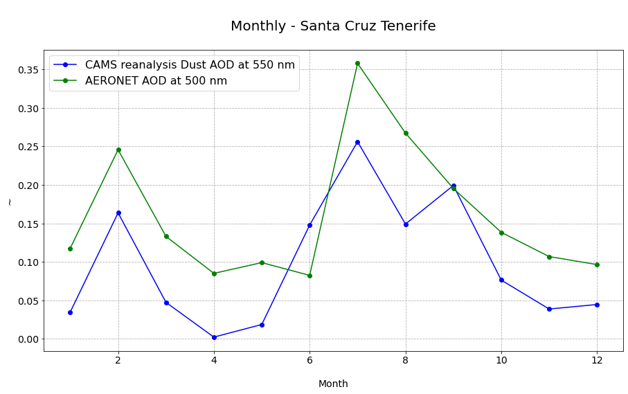
The monthly aggregates of AERONET observations and CAMS reanalysis follow a similar pattern for the year 2020.