Metop-A/B/C GOME-2 AAI product

Metop-A/B/C GOME-2 AAI product#

Hint

Execute the notebook on the training platform >>

The following example introduces you to the Absorbing Aerosol Index (AAI) Level 3 data product from the GOME-2 instrument onboard the three Metop satellites Metop-A/B/C. The Absorbing Aerosol Index (AAI) indicates the presence of elevated absorbing aerosols in the Earth’s atmosphere. The aerosol types that are mostly seen in the AAI are desert dust and biomass burning aerosols. The Absorbing Aerosol Index is derived from reflectances measured by GOME-2 at 340 and 380 nm. The data of the Metop-A/B/C GOME-2 Absorbing Aerosol Index (AAI) are provided by KNMI in the framework of the EUMETSAT Satellite Application Facility on Atmospheric Composition Monitoring (AC SAF).

Find more information on the GOME-2 Level 3 AAI data product processed by KNMI here.

Basic facts

Spatial resolution: 1° x 1°, gridded onto a regular lat-lon grid
Spatial coverage: Global
Temporal resolution: daily and monthly aggregates
Data availability: Metop-A: since 2007, Metop-B: since 2012, Metop-C: since 2019

How to access the data

GOME-2 AAI Level 3 data are available for download via TEMIS, a web-based service for atmospheric satellite data products maintained by KNMI. TEMIS provides daily and monthly aggregated Level 3 (gridded) data products for the three satellites Metop-A, -B, and -C.

To replicate the example below, you can go to the download page, select under GOME-2 / MetOp-A AAI daily gridded the year 2024 and then click on 5 April 2024. The download of the selected NetCDF file will start.

Load required libraries

import xarray as xr
import pandas as pd
from datetime import datetime

# Python libraries for visualisation
from matplotlib import pyplot as plt
from matplotlib import animation

import cartopy.crs as ccrs
from cartopy.mpl.gridliner import LONGITUDE_FORMATTER, LATITUDE_FORMATTER

from IPython.display import HTML

Load helper functions

%run ../../functions.ipynb

Load and browse Metop-A GOME-2 Level 3 AAI data#

The Metop-A/B/C GOME-3 Level 3 AAI data files can be downloaded from the TEMIS website in NetCDF data format. TEMIS offers the data of all three satellites Metop-A, -B and -C, which, combined, provide daily measurements for the entire globe.

The following example uses daily gridded AAI data from the three satellites Metop-A, -B, and -C for 3 consecutive days between 5 to 7 April 2024. The example shows the dispersion of aerosols during the Saharan dust event over part of south-east France, Switzerland and northern Italy.

Daily gridded data is available for each satellite. Thus, the first step is to inspect one file to get a better understanding of the general data structure. Followed by loading the data files for the entire time period into one xarray.DataArray and to repeat this for each of the three satellites Metop-A, -B and -C.

Inspect the structure of one daily gridded AAI data file

The data is in the folder ../../eodata/1_satellite/gome2/. Since the data is distributed in the NetCDF format, you can use the xarray function xr.open_dataset() to load one single file to better understand the data structure.

The output of the xarray.Dataset above shows that one file contains the data of three variables:

absorbing_aerosol_index,
number_of_observations, and
solar_zenith_angle.

The variable of interest is absorbing aerosol_index. By adding the variable of interest into square brackets [], you can select the data variable. Variables are stored as xarray.DataArray. You can see that the daily gridded data are on a 1 deg x 1 deg data grid, with 180 latitude values and 360 longitude values.

Load a time-series of daily Metop-A GOME-2 Level 3 AAI data into one xarray.Dataset

The xarray open_mfdataset() function allows the opening of multiple files at once. You have to specify the dimension the files shall be concatenated by. It can be an existing dimension within the data file or a new dimension, which is newly specified.

Let us open the daily gridded AAI data from Metop-B for the 3 days from 5 to 7 April 2024. We specify time as a new dimension that the data files shall be concatenated by. After you loaded the multiple files in a Dataset with the function open_mfdataset(), you have to select absorbing_aerosol_index again as the variable of interest.

The resulting xarray.DataArray has three dimensions (time, latitude and longitude).

ds_b = xr.open_mfdataset('../../eodata/1_satellite/gome2/20240408/ESACCI-AEROSOL-L3-AAI-GOME2B*', 
                         concat_dim='time', 
                         combine='nested')

aai_b=ds_b['absorbing_aerosol_index']
aai_b

<xarray.DataArray 'absorbing_aerosol_index' (time: 3, longitude: 360,
                                             latitude: 180)> Size: 778kB
dask.array<concatenate, shape=(3, 360, 180), dtype=float32, chunksize=(1, 360, 180), chunktype=numpy.ndarray>
Coordinates:
  * longitude  (longitude) float32 1kB -179.5 -178.5 -177.5 ... 178.5 179.5
  * latitude   (latitude) float32 720B -89.5 -88.5 -87.5 ... 87.5 88.5 89.5
Dimensions without coordinates: time
Attributes:
    long_name:  absorbing aerosol index averaged for each grid cell
    units:      1

The same process has to be repeated for the daily gridded AAI data from the satellites Metop-B and Metop-C respectively. Below, we load the GOME-2 Level 3 AAI data from the Metop-B satellite.

ds_c = xr.open_mfdataset('../../eodata/1_satellite/gome2/20240408/ESACCI-AEROSOL-L3-AAI-GOME2C*', 
                         concat_dim='time', 
                         combine='nested')

aai_c =ds_c['absorbing_aerosol_index']
aai_c

<xarray.DataArray 'absorbing_aerosol_index' (time: 3, longitude: 360,
                                             latitude: 180)> Size: 778kB
dask.array<concatenate, shape=(3, 360, 180), dtype=float32, chunksize=(1, 360, 180), chunktype=numpy.ndarray>
Coordinates:
  * longitude  (longitude) float32 1kB -179.5 -178.5 -177.5 ... 178.5 179.5
  * latitude   (latitude) float32 720B -89.5 -88.5 -87.5 ... 87.5 88.5 89.5
Dimensions without coordinates: time
Attributes:
    long_name:  absorbing aerosol index averaged for each grid cell
    units:      1

Concatenate the data from the two satellites Metop-B and -C#

The overall goal is to bring the AAI data from all three satellites together. Thus, the next step is to concatenate the DataArrays from the two satellites Metop-B and -C using a new dimension called satellite. You can use the concat() function from the xarray library to do this.

The result is a four-dimensional xarray.DataArray, with the dimensions satellite, time, latitude and longitude.

You can see that the resulting xarray.DataArray holds coordinate information for the two spatial dimensions longitude and latitude, but not for time and satellite.

However, the coordinates for time will be important for plotting the data as we need to know which day the data is valid. Thus, a next step is to assign coordinates to the time dimension.

aai_concat = xr.concat([aai_b,aai_c], dim='satellite')
aai_concat

<xarray.DataArray 'absorbing_aerosol_index' (satellite: 2, time: 3,
                                             longitude: 360, latitude: 180)> Size: 2MB
dask.array<concatenate, shape=(2, 3, 360, 180), dtype=float32, chunksize=(1, 1, 360, 180), chunktype=numpy.ndarray>
Coordinates:
  * longitude  (longitude) float32 1kB -179.5 -178.5 -177.5 ... 178.5 179.5
  * latitude   (latitude) float32 720B -89.5 -88.5 -87.5 ... 87.5 88.5 89.5
Dimensions without coordinates: satellite, time
Attributes:
    long_name:  absorbing aerosol index averaged for each grid cell
    units:      1

Assign time coordinates

By inspecting the metadata of the single data file aai_gome2b we loaded at the beginning, you can see that the only metadata attribute that contains the valid time step is the description attribute.

The first step is to retrieve the metadata attribute description and to split the resulting string object at the positions with a space. The day string is the fourth position of the resulting string.

The description attribute can be accessed directly from the aai_gome2b Dataset object.

start_day = aai_gome2b.description.split()[4]
start_day

'05-04-2024'

With the help of the Python library pandas, you can build a DateTime time series for the three consecutive days, starting from the start_day variable that was defined above.

You can use the date_range function from pandas, using the length of the time dimension of the aai_concat DataArray and 'd' (for day) as freqency argument.

The result is a time-series with DateTime information from 5 to 7 April 2024.

time_coords = pd.date_range(datetime.strptime(start_day,'%d-%m-%Y'), periods=len(aai_concat.time), freq='d').strftime("%Y-%m-%d").astype('datetime64[ns]')
time_coords

DatetimeIndex(['2024-04-05', '2024-04-06', '2024-04-07'], dtype='datetime64[ns]', freq=None)

The final step is to assign the pandas time series object time_coords to the aai_concat DataArray object. You can use the assign_coords() function from xarray. The result is that the time coordinates have now been assigned values. The only dimension the remains unassigned is satellite.

aai_concat = aai_concat.assign_coords(time=time_coords)
aai_concat

<xarray.DataArray 'absorbing_aerosol_index' (satellite: 2, time: 3,
                                             longitude: 360, latitude: 180)> Size: 2MB
dask.array<concatenate, shape=(2, 3, 360, 180), dtype=float32, chunksize=(1, 1, 360, 180), chunktype=numpy.ndarray>
Coordinates:
  * longitude  (longitude) float32 1kB -179.5 -178.5 -177.5 ... 178.5 179.5
  * latitude   (latitude) float32 720B -89.5 -88.5 -87.5 ... 87.5 88.5 89.5
  * time       (time) datetime64[ns] 24B 2024-04-05 2024-04-06 2024-04-07
Dimensions without coordinates: satellite
Attributes:
    long_name:  absorbing aerosol index averaged for each grid cell
    units:      1

Combine AAI data from the two satellites onto one single grid

Since the final aim is to combine the data from the two satellites Metop-B and -C onto one single grid, the next step is to reduce the satellite dimension. You can do this by applying the reduce function mean to the aai_concat Data Array. The dimension (dim) to be reduced is the satellite dimension.

This function builds the average of all data points within a grid cell. The resulting xarray.DataArray has three dimensions time, latitude and longitude.

aai_combined = aai_concat.mean(dim='satellite')
aai_combined

<xarray.DataArray 'absorbing_aerosol_index' (time: 3, longitude: 360,
                                             latitude: 180)> Size: 778kB
dask.array<mean_agg-aggregate, shape=(3, 360, 180), dtype=float32, chunksize=(1, 360, 180), chunktype=numpy.ndarray>
Coordinates:
  * longitude  (longitude) float32 1kB -179.5 -178.5 -177.5 ... 178.5 179.5
  * latitude   (latitude) float32 720B -89.5 -88.5 -87.5 ... 87.5 88.5 89.5
  * time       (time) datetime64[ns] 24B 2024-04-05 2024-04-06 2024-04-07

Visualize GOME-2 AAI data from the two satellites Metop-B and C combined on one grid#

The next step is to visualize the Absorbing Aerosol Index data for one time step. You can use the function visualize_pcolormesh for it.

You can use afmhot_r as color map, ccrs.PlateCarree() as projection and by applying dt.strftime('%Y-%m-%d').data to the time coordinate variable, you can add the valid time step to the title of the plot.

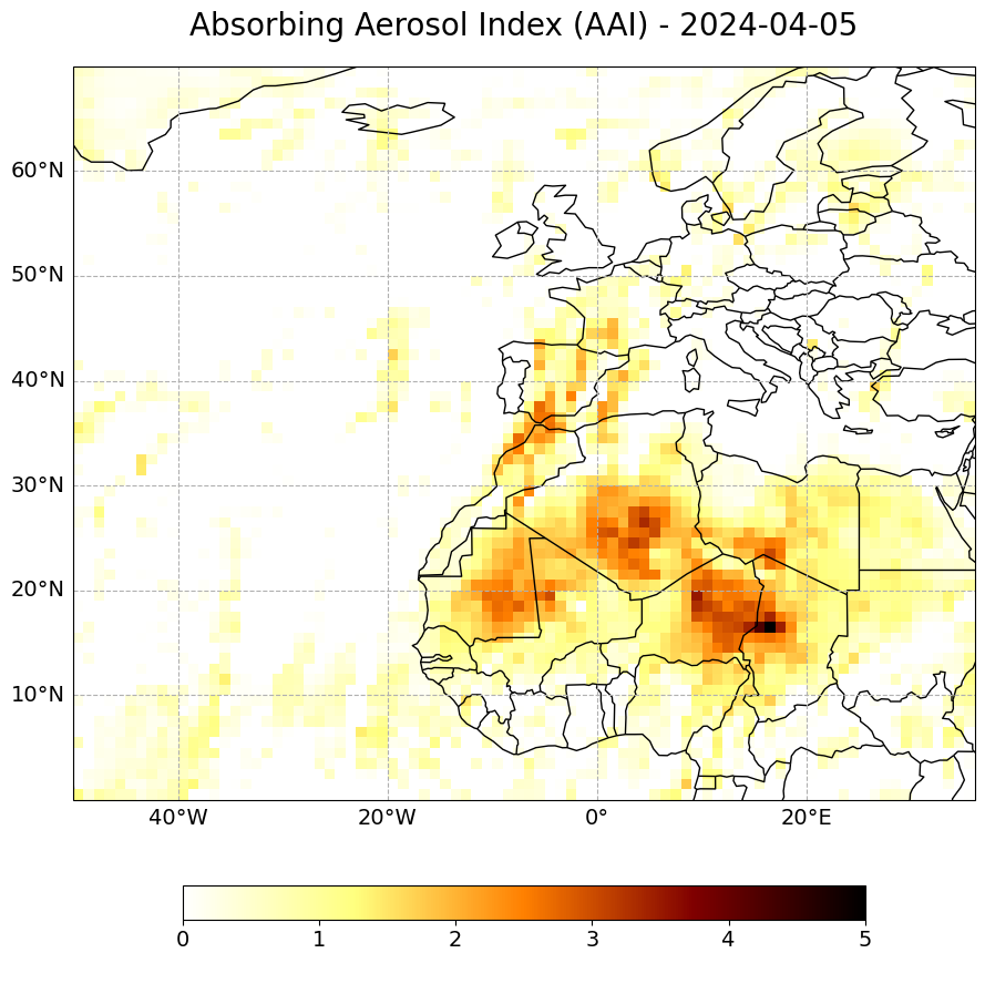
The resulting plot shows elevated AAI levels over Spain and wester Mediterranean on 7 April 2024.

visualize_pcolormesh(data_array=aai_combined[2,:,:].T,
                     longitude=aai_combined.longitude, 
                     latitude=aai_combined.latitude,
                     projection=ccrs.PlateCarree(), 
                     color_scale='afmhot_r', 
                     unit=' ',
                     long_name='Absorbing Aerosol Index (AAI) - ' + str(aai_combined.time[0].dt.strftime('%Y-%m-%d').data)[0:10], 
                     vmin=0, 
                     vmax=5, 
                     lonmin=-50, 
                     lonmax=36, 
                     latmin=0, 
                     latmax=70.,
                     set_global=False)

(<Figure size 2000x1000 with 2 Axes>,
 <GeoAxes: title={'center': 'Absorbing Aerosol Index (AAI) - 2024-04-05'}>)

../_images/6e511611f02f7f28c1c8afe12cdba7ef6a4795d6eab50660f7b1c4902b694424.png

Animate daily Metop-B/C GOME-2 L3 AAI data between 5 to 7 April 2024#

The final step is now to animate the aai_combined DataArray over the 3 days to see the dispersion of Aerosols resulting from the Saharan dust event over Spain and the western Mediterranean in April 2024.

The animation function consists of four parts:

Setting the initial state:
Here, you define the general plot your animation shall use to initialise the animation. You can also define the number of frames (time steps) your animation shall have.
Functions to animate:
An animation consists of three functions: draw(), init() and animate(). draw() is the function where individual frames are passed on and the figure is returned as image. In this example, the function redraws the plot for each time step. init() returns the figure you defined for the initial state. animate() returns the draw() function and animates the function over the given number of frames (time steps).
Create a animate.FuncAnimation object:
The functions defined before are now combined to build an animate.FuncAnimation object.
Play the animation as video:
As a final step, you can integrate the animation into the notebook with the HTML class. You take the generate animation object and convert it to a HTML5 video with the to_html5_video function

# Setting the initial state:
# 1. Define figure for initial plot
fig, ax = visualize_pcolormesh(data_array=aai_combined[0,:,:].T,
                               longitude=aai_combined.longitude, 
                               latitude=aai_combined.latitude,
                               projection=ccrs.PlateCarree(), 
                               color_scale='afmhot_r', 
                               unit=' ',
                               long_name='Absorbing Aerosol Index (AAI) - ' + str(aai_combined.time[0].dt.strftime('%Y-%m-%d').data)[0:10], 
                               vmin=0, 
                               vmax=6, 
                               lonmin=-20, 
                               lonmax=36, 
                               latmin=20, 
                               latmax=70.,
                               set_global=False)

frames = 3

def draw(i):
    img = plt.pcolormesh(aai_combined.longitude, 
                         aai_combined.latitude, 
                         aai_combined[i,:,:].T, 
                         cmap='afmhot_r', 
                         transform=ccrs.PlateCarree(),
                         vmin=0,
                         vmax=6)
    ax.set_title('Absorbing Aerosol Index (AAI) - ' + str(aai_combined.time[i].dt.strftime('%Y-%m-%d').data)[0:10],
                fontsize=20, pad=20.0)
    return img

def init():
    return fig

def animate(i):
    return draw(i)

ani = animation.FuncAnimation(fig, animate, frames, interval=800, blit=False,
                              init_func=init, repeat=True)

HTML(ani.to_html5_video())
plt.close(fig)

Play the animation as HTML5 video

HTML(ani.to_html5_video())