Solution 1

Hint

Execute the notebook on the training platform >>

About

You are working for ENAIRE, the air navigation authority for Spain and western Africa. You know that the Canary Islands are prone to Saharan dust events and for this reason, ENAIRE monitors dust on a daily basis. You are the operations analyst for the week of 21-27 February 2020 and responsible for issuing alerts, and if necessary, to mandate required safety measures.

On 21 February 2020, you are in-charge of analysing the dust forecast and to monitor potential dust events for the coming days. With your new knowledge on aerosol and dust data, you should be able to do this.

Tasks

1. Brainstorm

• What dust forecasts do you know about?

• How do they differ from each other?

• What satellite data do you know about that can be used for dust nowcasting?

• Which variables can be used to monitor and forecast dust?

2. Download and animate the MONARCH dust forecast

• Download the dust forecast from the MONARCH model for 21 February 2020 and animate the forecast

• Hint

  • WMO SDS-WAS dust forecast - Example notebook

  • Data access (Username: sdswas.namee.rc@gmail.com, Password: BarcelonaDustRC)

3. Download the MSG SEVIRI Level 1.5 data and visualize the Dust RGB composite

• Based on the dust forecast for the next days - which day and hour would you choose for getting a near real-time monitoring of dust from the MSG SEVIRI instrument?

• Hint

  • MSG SEVIRI Level 1.5 - Example notebook

  • Data access

4. Interpret the results

• Describe the dust forecast event in comparison with the near real-time monitoring from the satellite.

• What decision as ENAIRE operations analyst do you take? Would you issue an alert? Would you implement some safety measures?

---

Load required libraries

import xarray as xr
import glob

from IPython.display import HTML

import matplotlib.pyplot as plt
import matplotlib.colors
from matplotlib.cm import get_cmap
from matplotlib import animation
from matplotlib.axes import Axes

import cartopy.crs as ccrs
from cartopy.mpl.gridliner import LONGITUDE_FORMATTER, LATITUDE_FORMATTER
import cartopy.feature as cfeature
from cartopy.mpl.geoaxes import GeoAxes
GeoAxes._pcolormesh_patched = Axes.pcolormesh

from satpy.scene import Scene
from satpy.composites import GenericCompositor
from satpy.writers import to_image
from satpy.resample import get_area_def
from satpy import available_readers

import pyresample

import warnings
warnings.simplefilter(action = "ignore", category = RuntimeWarning)

Load helper functions

%run ../../functions.ipynb

---

1. Brainstorm

Model forecasts

• MONARCH regional dust forecasts

• CAMS European air quality forecasts and analyses

• CAMS global atmospheric composition forecast

Forecast models differ in their spatial and temporal resolution, but also spatial coverage and forecast period.

Satellite observations

• MSG SEVIRI Level 1 RGB composites

• Terra/Aqua MODIS Level 1 RGB composites

The following variables can be used to monitor and forecast dust:

• Dust Optical Depth

• Aerosol Optical Depth

2. Download and animate the MONARCH dust forecast

The first step is to load a MONARCH forecast file. The data is disseminated in the netCDF format on a daily basis, with the forecast initialisation at 12:00 UTC. Load the MONARCH dust forecast of 21 February 2020. You can use the function open_dataset() from the xarray Python library.

Once loaded, you see that the data has three dimensions: lat, lon and time; and offers two data variables od550_dust and sconc_dust.

filepath = '../../eodata/case_study/sds_was/2020022112_3H_NMMB-BSC.nc'
file = xr.open_dataset(filepath)
file

<xarray.Dataset>
Dimensions:     (lon: 307, lat: 211, time: 25)
Coordinates:
  * lon         (lon) float64 -31.0 -30.67 -30.33 -30.0 ... 70.33 70.67 71.0
  * lat         (lat) float64 -3.0 -2.667 -2.333 -2.0 ... 66.0 66.33 66.67 67.0
  * time        (time) datetime64[ns] 2020-02-21T12:00:00 ... 2020-02-24T12:0...
Data variables:
    od550_dust  (time, lat, lon) float32 ...
    sconc_dust  (time, lat, lon) float32 ...
Attributes:
    CDI:                       Climate Data Interface version 1.5.4 (http://c...
    Conventions:               CF-1.2
    history:                   Fri Feb 21 23:50:54 2020: cdo remapbil,regular...
    _FillValue:                -32767.0
    missing_value:             -32767.0
    title:                     Regional Reanalysis 0.5x0.5 deg NMMB-BSC-Dust ...
    History:                   Fri Feb 21 22:12:45 2020: ncrcat -F -O pout_re...
    Grid_type:                 B-grid: vectors interpolated to scalar positions
    Map_Proj:                  Rotated latitude longitude
    NCO:                       4.0.8
    nco_openmp_thread_number:  1
    CDO:                       Climate Data Operators version 1.5.4 (http://c...

Let us then retrieve the data variable od550_dust, which is the dust optical depth at 550 nm.

od550_dust = file['od550_dust']
od550_dust

<xarray.DataArray 'od550_dust' (time: 25, lat: 211, lon: 307)>
[1619425 values with dtype=float32]
Coordinates:
  * lon      (lon) float64 -31.0 -30.67 -30.33 -30.0 ... 70.0 70.33 70.67 71.0
  * lat      (lat) float64 -3.0 -2.667 -2.333 -2.0 ... 66.0 66.33 66.67 67.0
  * time     (time) datetime64[ns] 2020-02-21T12:00:00 ... 2020-02-24T12:00:00
Attributes:
    long_name:  dust optical depth at 550 nm
    units:       
    title:      dust optical depth at 550 nm

Let us now have a closer look at the dimensions of the data. Let us first inspect the two coordinate dimensions lat and lon. You can simply access the dimension’s xarray.DataArray by specifying the name of the dimension. Below you see that the data has a 0.1 x 0.1 degrees resolution and have the following geographical bounds:

• Longitude: [-63., 101.9]

• Latitude: [-11., 71.4]

latitude = file.lat
longitude = file.lon
latitude, longitude

(<xarray.DataArray 'lat' (lat: 211)>
 array([-3.      , -2.666667, -2.333333, ..., 66.333326, 66.66666 , 66.999993])
 Coordinates:
   * lat      (lat) float64 -3.0 -2.667 -2.333 -2.0 ... 66.0 66.33 66.67 67.0
 Attributes:
     standard_name:  latitude
     long_name:      latitude
     units:          degrees_north
     axis:           Y,
 <xarray.DataArray 'lon' (lon: 307)>
 array([-31.      , -30.666667, -30.333333, ...,  70.333323,  70.666657,
         70.99999 ])
 Coordinates:
   * lon      (lon) float64 -31.0 -30.67 -30.33 -30.0 ... 70.0 70.33 70.67 71.0
 Attributes:
     standard_name:  longitude
     long_name:      longitude
     units:          degrees_east
     axis:           X)

Now, let us also inspect the time dimension. You see that one daily forecast file has 25 time steps, with three hourly forecast information up to 72 hours (3 days) in advance.

file.time

<xarray.DataArray 'time' (time: 25)>
array(['2020-02-21T12:00:00.000000000', '2020-02-21T15:00:00.000000000',
       '2020-02-21T18:00:00.000000000', '2020-02-21T21:00:00.000000000',
       '2020-02-22T00:00:00.000000000', '2020-02-22T03:00:00.000000000',
       '2020-02-22T06:00:00.000000000', '2020-02-22T09:00:00.000000000',
       '2020-02-22T12:00:00.000000000', '2020-02-22T15:00:00.000000000',
       '2020-02-22T18:00:00.000000000', '2020-02-22T21:00:00.000000000',
       '2020-02-23T00:00:00.000000000', '2020-02-23T03:00:00.000000000',
       '2020-02-23T06:00:00.000000000', '2020-02-23T09:00:00.000000000',
       '2020-02-23T12:00:00.000000000', '2020-02-23T15:00:00.000000000',
       '2020-02-23T18:00:00.000000000', '2020-02-23T21:00:00.000000000',
       '2020-02-24T00:00:00.000000000', '2020-02-24T03:00:00.000000000',
       '2020-02-24T06:00:00.000000000', '2020-02-24T09:00:00.000000000',
       '2020-02-24T12:00:00.000000000'], dtype='datetime64[ns]')
Coordinates:
  * time     (time) datetime64[ns] 2020-02-21T12:00:00 ... 2020-02-24T12:00:00
Attributes:
    standard_name:  time

You can define variables for the attributes of a variable. This can be helpful during data visualization, as the attributes long_name and units can be added as additional information to the plot. From the xarray.DataArray, you simply specify the name of the attribute of interest.

long_name=od550_dust.long_name
units= od550_dust.units

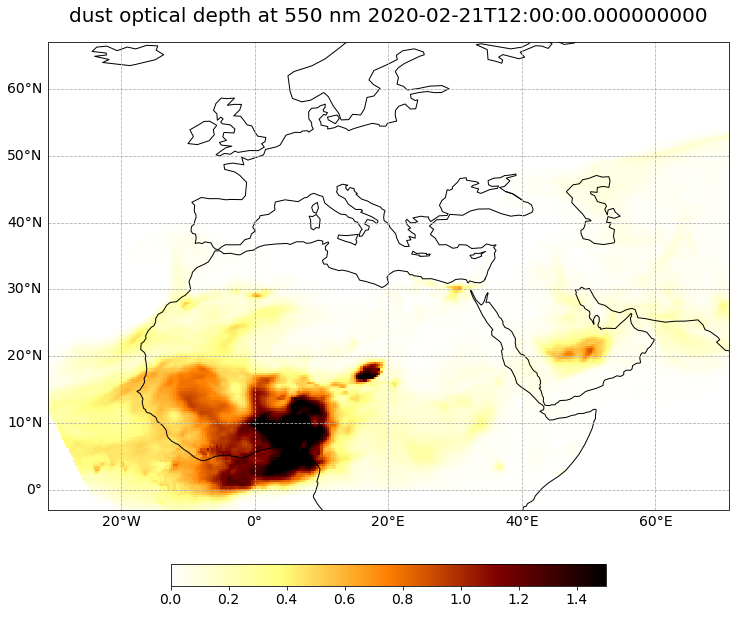
Visualize dust Aerosol Optical Depth

Now we have loaded all necessary information to be able to visualize the dust Aerosol Optical Depth for one specific time during the forecast run. Let us use the function visualize_pcolormesh() to visualize the data with the help of the plotting library matplotlib and Cartopy.

You have to specify the following keyword arguments:

• data_array: the

• longitude, latitude: longitude and latitude variables of the data variable

• projection: one of Cartopy’s projection options

• color_scale: one of matplotlib’s colormaps

• units: unit of the data parameter, preferably taken from the data array’s attributes

• long_name: longname of the data parameter is taken as title of the plot, preferably taken from the data array’s attributes

• vmin, vmax: minimum and maximum bounds of the color range

• set_global: False, if data is not global

• lonmin, lonmax, latmin, latmax: kwargs have to be specified, if set_global=False

Note: in order to have the time information as part of the title, we add the string of the datetime information to the long_name variable: long_name + ' ' + str(od_dust[##,:,:].time.data).

forecast_step=0
visualize_pcolormesh(data_array=od550_dust[forecast_step,:,:],
                     longitude=od550_dust.lon,
                     latitude=od550_dust.lat,
                     projection=ccrs.PlateCarree(),
                     color_scale='afmhot_r',
                     unit=units,
                     long_name=long_name + ' ' + str(od550_dust[forecast_step,:,:].time.data),
                     vmin=0, 
                     vmax=1.5,
                     set_global=False,
                     lonmin=longitude.min().data,
                     lonmax=longitude.max().data,
                     latmin=latitude.min().data,
                     latmax=latitude.max().data)

(<Figure size 1440x720 with 2 Axes>,
 <GeoAxesSubplot:title={'center':'dust optical depth at 550 nm 2020-02-21T12:00:00.000000000'}>)

Animate dust Aerosol Optical Depth forecasts

In the last step, you can animate the Dust Aerosol Optical Depth forecasts in order to see how the trace gas develops over a period of 3 days, from 20th Feb 12 UTC to 24th February 2021.

You can do animations with matplotlib’s function animation. Jupyter’s function HTML can then be used to display HTML and video content.

The animation function consists of 4 parts:

• Setting the initial state:
  Here, you define the general plot your animation shall use to initialise the animation. You can also define the number of frames (time steps) your animation shall have.

• Functions to animate:
  An animation consists of three functions: draw(), init() and animate(). draw() is the function where individual frames are passed on and the figure is returned as image. In this example, the function redraws the plot for each time step. init() returns the figure you defined for the initial state. animate() returns the draw() function and animates the function over the given number of frames (time steps).

• Create a animate.FuncAnimation object:
  The functions defined before are now combined to build an animate.FuncAnimation object.

• Play the animation as video:
  As a final step, you can integrate the animation into the notebook with the HTML class. You take the generate animation object and convert it to a HTML5 video with the to_html5_video function

# Setting the initial state:
# 1. Define figure for initial plot
fig, ax = visualize_pcolormesh(data_array=od550_dust[0,:,:],
                     longitude=od550_dust.lon,
                     latitude=od550_dust.lat,
                     projection=ccrs.PlateCarree(),
                     color_scale='afmhot_r',
                     unit=units,
                     long_name=long_name + ' ' + str(od550_dust[0,:,:].time.data),
                     vmin=0, 
                     vmax=1.5,
                     lonmin=longitude.min().data,
                     lonmax=longitude.max().data,
                     latmin=latitude.min().data,
                     latmax=latitude.max().data,
                     set_global=False)

frames = 24

def draw(i):
    img = plt.pcolormesh(od550_dust.lon, 
                         od550_dust.lat, 
                         od550_dust[i,:,:], 
                         cmap='afmhot_r', 
                         transform=ccrs.PlateCarree(),
                         vmin=0,
                         vmax=1.5,
                         shading='auto')
    
    ax.set_title(long_name + ' '+ str(od550_dust.time[i].data), fontsize=20, pad=20.0)
    return img


def init():
    return fig


def animate(i):
    return draw(i)

ani = animation.FuncAnimation(fig, animate, frames, interval=800, blit=False,
                              init_func=init, repeat=True)

HTML(ani.to_html5_video())
plt.close(fig)

HTML(ani.to_html5_video())

---

3. Download the MSG SEVIRI Level 1.5 data and visualize the Dust RGB composite

From the EUMETSAT Data Store, we downloaded High Rate SEVIRI Level 1.5 Image data for 23 February 2020 at 18 UTC.

The data is downloaded as a zip archive. We already unzipped the file. Hence, in a next step we can specify the file path and create a variable with the name file_name.

file_name = glob.glob('../../eodata/case_study/meteosat/event/2020/02/23/MSG4-SEVI-MSG15-0100-NA-20200223181244.112000000Z-NA.nat')
file_name

['../../eodata/case_study/meteosat/event/2020/02/23/MSG4-SEVI-MSG15-0100-NA-20200223181244.112000000Z-NA.nat']

In a next step, we use the Scene constructor from the satpy library. Once loaded, a Scene object represents a single geographic region of data, typically at a single continuous time range.

You have to specify the two keyword arguments reader and filenames in order to successfully load a scene. As mentioned above, for MSG SEVIRI data in the Native format, you can use the seviri_l1b_native reader.

scn = Scene(reader="seviri_l1b_native", 
             filenames=file_name)
scn

<satpy.scene.Scene at 0x7f7c2c5fb340>

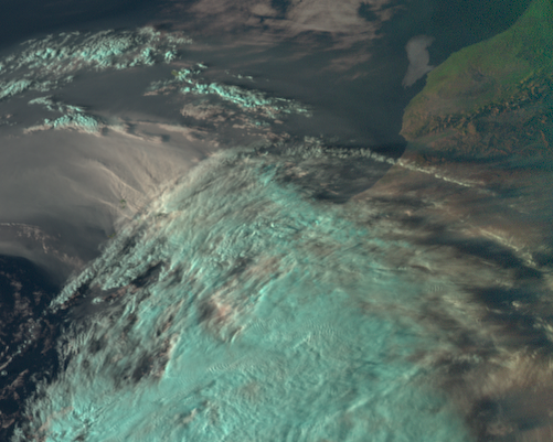
Load the RGB composite ID natural color

Let us define load the composite ID natural_color. This list variable can then be passed to the function load(). Per default, scenes are loaded with the north pole facing downwards. You can specify the keyword argument upper_right_corner=NE in order to turn the image around and have the north pole facing upwards.

composite_id = ["natural_color"]
scn.load(composite_id, upper_right_corner="NE")

A print of the Scene object scn shows you that one band is available: natural_color

print(scn)

<xarray.DataArray 'where-1eeee2327f1f52a84787d02280871d42' (bands: 3, y: 3712, x: 3712)>
dask.array<where, shape=(3, 3712, 3712), dtype=float32, chunksize=(1, 3712, 3712), chunktype=numpy.ndarray>
Coordinates:
    crs      object PROJCRS["unknown",BASEGEOGCRS["unknown",DATUM["unknown",E...
  * y        (y) float64 5.569e+06 5.566e+06 5.563e+06 ... -5.563e+06 -5.566e+06
  * x        (x) float64 -5.569e+06 -5.566e+06 ... 5.563e+06 5.566e+06
  * bands    (bands) <U1 'R' 'G' 'B'
Attributes:
    end_time:                               2020-02-23 18:15:11.171248
    sun_earth_distance_correction_factor:   0.9787042740413612
    start_time:                             2020-02-23 18:00:11.057487
    area:                                   Area ID: msg_seviri_fes_3km\nDesc...
    georef_offset_corrected:                True
    orbital_parameters:                     {'projection_longitude': 0.0, 'pr...
    reader:                                 seviri_l1b_native
    sensor:                                 seviri
    ancillary_variables:                    []
    standard_name:                          natural_color
    resolution:                             3000.403165817
    platform_name:                          Meteosat-11
    sun_earth_distance_correction_applied:  True
    wavelength:                             None
    optional_datasets:                      []
    name:                                   natural_color
    _satpy_id:                              DataID(name='natural_color', reso...
    prerequisites:                          [DataQuery(name='IR_016', modifie...
    optional_prerequisites:                 []
    mode:                                   RGB

Generate a geographical subset over Canary Islands

Crop the data with x and y values in original projection unit (x_min, y_min, x_max, y_max). Below we apply the funcion crop() and use the keyword argument xy_bbox=(xmin, ymin, xmax, ymax) in order to crop the file based on an area in original projection unit. For the bbox information we use the following settings: xmin=-20E5, ymin=23E5, xmax=-5E5, ymax=35E5.

Then, let’s visualize the cropped image with the function show().

scn_cropped = scn.crop(xy_bbox=(-20E5, 23E5, -5E5, 35E5))
scn_cropped.show("natural_color")

Let us store the area definition as variable.

area = scn_cropped['natural_color'].attrs['area']
area

Next, use the area definition to resample the loaded Scene object. Afterwards, you can visualize the resampled image with the function show().

scn_resample_nc = scn.resample(area)
scn_resample_nc.show('natural_color')

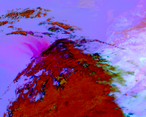
Load, visualize and interpret the MSG SEVIRI Dust RGB composite

Let us reload the file with the Scene constructor.

scn2 = Scene(reader="seviri_l1b_native", 
             filenames=file_name)
scn2

<satpy.scene.Scene at 0x7f7d387b6bb0>

Let us define a composite ID for dust in a list. This list variable can then be passed to the function load(). Per default, scenes are loaded with the north pole facing downwards. You can specify the keyword argument upper_right_corner=NE in order to turn the image around and have the north pole facing upwards.

composite_id = ["dust"]
scn2.load(composite_id, upper_right_corner="NE")

Next, use the same area definition to resample the loaded Scene object.

scn2_resample_nc = scn2.resample(area)

Afterwards, you can visualize the resampled image with the function show().

scn2_resample_nc.show('dust')