Solution 3#
About#
With exercise #1 and exercise #2, you compared two dust forecast models as well as near real-time monitoring with satellite data. From the results of the assignment, you see that it is difficult to know which forecast can be trusted more. Hence, even though model intercomparison is important, model outcomes also have to be compared with real-world observations. Just by comparing model outcomes with measurements from station data, we can better understand how the model performs.
Now, you will focus on how you can use station observations from AERONET to evaluate model forecasts.
Tasks#
1. Brainstorm
What observation datasets do you know about?
Which variables do they measure?
Which data can you use to evaluate model predictions?
2. Download and plot time-series of AERONET data for Santa Cruz, Tenerife
Download and visualise AERONET v3.0 measurements of the station Santa Cruz, Tenerife for 21 to 25 February 2020.
Some questions to reflect on:
Under which name is the station listed in AERONET?
What average level would you choose?
Which days do we have observations for?
Hint
3. Resample AERONET data to a 3-hourly resolution
Make use of AERONET
indexandtimecolumns to create aDateTimeIndexin order to resample the observations to a 3-hourly temporal resolutionHint
you have to combine the two columns
indexandtimeas one string variableyou can use the pandas function
to_datetime()to create aDateTimeIndexand the functionresample().mean()to resample and average the time-series to a given temporal resolution
Question to reflect on
How many row entries does the resampled data frame have?
4. Load time-series of the forecasts from CAMS and the MONARCH model and compare it with the AERONET observations
Interpret the plotting result.
Can you make a statement of the performance of the two forecast models?
What is your conclusion regarding AERONET observation data?
Load required libraries
import wget
import pandas as pd
import numpy as np

import matplotlib.pyplot as plt
import matplotlib.colors
from matplotlib.cm import get_cmap
from matplotlib import animation
from matplotlib.axes import Axes

import cartopy.crs as ccrs
from cartopy.mpl.gridliner import LONGITUDE_FORMATTER, LATITUDE_FORMATTER
import cartopy.feature as cfeature
from cartopy.mpl.geoaxes import GeoAxes
GeoAxes._pcolormesh_patched = Axes.pcolormesh

import warnings
warnings.simplefilter(action = "ignore", category = RuntimeWarning)
Load helper functions
%run ../../functions.ipynb
1. Brainstorm#
Three different ground-based observations are introduced during the course:
-
Aerosol Optical Depth
Angstrom Exponent
EARLINET Lidar backscatter profiles
Backscatter coefficient
-
PM2.5
PM10
AERONET offers ground-based observations of Aerosol Optical Depth and the Angstrom Exponent and can be used to evaluate dust forecasts.
2. Download and plot time-series of AERONET data#
Define the latitude / longitude values for Santa Cruz, Tenerife. You can see an overview of all available AERONET Site Names here.
lat = 28.473
lon = -16.247
As a first step, let us create a Python dictionary in which we store all the parameters we would like to use for the request as dictionary keys. You can initiate a dictionary with curled brackets {}. Below, we specify the following parameters:
endpoint: Endpoint of the AERONET web servicestation: Name of the AERONET stationyear: year 1 of interestmonth: month 1 of interestday: day 1 of interestyear2: year 2 of interestmonth2: month 2 of interestday2: day 2 of interestAOD15: data type, other options includeAOD10,AOD20, etc.AVG: data format,AVG=10- all points,AVG=20- daily averages
The keywords below are those we will need for requesting all data points (AVG=10) of Aerosol Optical Depth Level 1.5 data for the station Santa Cruz, Tenerife for 21 to 25 February 2020.
data_dict = {
    'endpoint': 'https://aeronet.gsfc.nasa.gov/cgi-bin/print_web_data_v3',
    'station':'Santa_Cruz_Tenerife',
    'year': 2020,
    'month': 2,
    'day': 21,
    'year2': 2020,
    'month2': 2,
    'day2': 25,
    'AOD15': 1,
    'AVG': 10
}
In a next step, we construct the final string for the wget request with the format function. You construct a string by adding the dictionary keys in curled brackets. At the end of the string, you provide the dictionary key informatoin to the string with the format() function. A print of the resulting url shows, that the format function replaced the information in the curled brackets with the data in the dictionary.
url = '{endpoint}?site={station}&year={year}&month={month}&day={day}&year2={year2}&month2={month2}&day2={day2}&AOD15={AOD15}&AVG={AVG}'.format(**data_dict)
url
'https://aeronet.gsfc.nasa.gov/cgi-bin/print_web_data_v3?site=Santa_Cruz_Tenerife&year=2020&month=2&day=21&year2=2020&month2=2&day2=25&AOD15=1&AVG=10'
Now we are ready to request the data with the function download() from the wget Python library. You have to pass to the function the constructed url above together with a file path of where the downloaded that shall be stored. Let us store the data as txt file in the folder ../data/2_observations/aeronet/.
wget.download(url, '../../../../eodata/50_modules/01_dust/04_assignment/aeronet/20200221-25_santa_cruz_tenerife_10.txt')
'../data/aeronet/20200221-25_santa_cruz_tenerife_10 (1).txt'
After we downloaded the station observations as txt file, we can open it with the pandas function read_table(). We additonally set specific keyword arguments that allow us to specify the columns and rows of interest:
delimiter: specify the delimiter in the text file, e.g. commaheader: specify the index of the row that shall be set as header.index_col: specify the index of the column that shall be set as index
You see below that the resulting dataframe has 292 rows and 113 columns.
df = pd.read_table('../../../../eodata/50_modules/01_dust/04_assignment/aeronet/20200221-25_santa_cruz_tenerife_10.txt', delimiter=',', header=[7], index_col=1)
df
| AERONET_Site | Time(hh:mm:ss) | Day_of_Year | Day_of_Year(Fraction) | AOD_1640nm | AOD_1020nm | AOD_870nm | AOD_865nm | AOD_779nm | AOD_675nm | ... | Exact_Wavelengths_of_AOD(um)_380nm | Exact_Wavelengths_of_AOD(um)_340nm | Exact_Wavelengths_of_PW(um)_935nm | Exact_Wavelengths_of_AOD(um)_681nm | Exact_Wavelengths_of_AOD(um)_709nm | Exact_Wavelengths_of_AOD(um)_Empty | Exact_Wavelengths_of_AOD(um)_Empty.1 | Exact_Wavelengths_of_AOD(um)_Empty.2 | Exact_Wavelengths_of_AOD(um)_Empty.3 | Exact_Wavelengths_of_AOD(um)_Empty<br> | |
|---|---|---|---|---|---|---|---|---|---|---|---|---|---|---|---|---|---|---|---|---|---|
| Date(dd:mm:yyyy) | |||||||||||||||||||||
| 21:02:2020 | Santa_Cruz_Tenerife | 08:22:46 | 52.0 | 52.349144 | 0.021395 | 0.031387 | 0.034429 | -999.0 | -999.0 | 0.040873 | ... | 0.3797 | 0.3398 | 0.9371 | -999.0 | -999.0 | -999.0 | -999.0 | -999.0 | -999.0 | -999.<br> |
| 21:02:2020 | Santa_Cruz_Tenerife | 08:25:22 | 52.0 | 52.350949 | 0.019840 | 0.028373 | 0.030877 | -999.0 | -999.0 | 0.035930 | ... | 0.3797 | 0.3398 | 0.9371 | -999.0 | -999.0 | -999.0 | -999.0 | -999.0 | -999.0 | -999.<br> |
| 21:02:2020 | Santa_Cruz_Tenerife | 08:28:46 | 52.0 | 52.353310 | 0.019732 | 0.028353 | 0.030869 | -999.0 | -999.0 | 0.035813 | ... | 0.3797 | 0.3398 | 0.9371 | -999.0 | -999.0 | -999.0 | -999.0 | -999.0 | -999.0 | -999.<br> |
| 21:02:2020 | Santa_Cruz_Tenerife | 08:30:39 | 52.0 | 52.354618 | 0.019704 | 0.028210 | 0.030609 | -999.0 | -999.0 | 0.035490 | ... | 0.3797 | 0.3398 | 0.9371 | -999.0 | -999.0 | -999.0 | -999.0 | -999.0 | -999.0 | -999.<br> |
| 21:02:2020 | Santa_Cruz_Tenerife | 08:33:09 | 52.0 | 52.356354 | 0.020827 | 0.030963 | 0.030745 | -999.0 | -999.0 | 0.035596 | ... | 0.3797 | 0.3398 | 0.9371 | -999.0 | -999.0 | -999.0 | -999.0 | -999.0 | -999.0 | -999.<br> |
| ... | ... | ... | ... | ... | ... | ... | ... | ... | ... | ... | ... | ... | ... | ... | ... | ... | ... | ... | ... | ... | ... |
| 25:02:2020 | Santa_Cruz_Tenerife | 18:09:31 | 56.0 | 56.756609 | 0.266426 | 0.359000 | 0.381361 | -999.0 | -999.0 | 0.412116 | ... | 0.3797 | 0.3398 | 0.9371 | -999.0 | -999.0 | -999.0 | -999.0 | -999.0 | -999.0 | -999.<br> |
| 25:02:2020 | Santa_Cruz_Tenerife | 18:13:14 | 56.0 | 56.759190 | 0.279673 | 0.374916 | 0.398722 | -999.0 | -999.0 | 0.430402 | ... | 0.3797 | 0.3398 | 0.9371 | -999.0 | -999.0 | -999.0 | -999.0 | -999.0 | -999.0 | -999.<br> |
| 25:02:2020 | Santa_Cruz_Tenerife | 18:15:09 | 56.0 | 56.760521 | 0.286610 | 0.384756 | 0.408843 | -999.0 | -999.0 | 0.440872 | ... | 0.3797 | -999.0000 | 0.9371 | -999.0 | -999.0 | -999.0 | -999.0 | -999.0 | -999.0 | -999.<br> |
| 25:02:2020 | Santa_Cruz_Tenerife | 18:17:13 | 56.0 | 56.761956 | 0.293157 | 0.393598 | 0.418218 | -999.0 | -999.0 | 0.451127 | ... | 0.3797 | -999.0000 | 0.9371 | -999.0 | -999.0 | -999.0 | -999.0 | -999.0 | -999.0 | -999.<br> |
| NaN | </body></html> | NaN | NaN | NaN | NaN | NaN | NaN | NaN | NaN | NaN | ... | NaN | NaN | NaN | NaN | NaN | NaN | NaN | NaN | NaN | NaN |
292 rows × 113 columns
Now, we can inspect the entries in the loaded data frame a bit more. Above you see that the last entry is a NaN entry, which is best to drop with the function dropna().
The next step is then to replace the entries with -999.0 and set them as NaN. We can use the function replace() to do so.
df = df.dropna()
df = df.replace(-999.0, np.nan)
df
| AERONET_Site | Time(hh:mm:ss) | Day_of_Year | Day_of_Year(Fraction) | AOD_1640nm | AOD_1020nm | AOD_870nm | AOD_865nm | AOD_779nm | AOD_675nm | ... | Exact_Wavelengths_of_AOD(um)_380nm | Exact_Wavelengths_of_AOD(um)_340nm | Exact_Wavelengths_of_PW(um)_935nm | Exact_Wavelengths_of_AOD(um)_681nm | Exact_Wavelengths_of_AOD(um)_709nm | Exact_Wavelengths_of_AOD(um)_Empty | Exact_Wavelengths_of_AOD(um)_Empty.1 | Exact_Wavelengths_of_AOD(um)_Empty.2 | Exact_Wavelengths_of_AOD(um)_Empty.3 | Exact_Wavelengths_of_AOD(um)_Empty<br> | |
|---|---|---|---|---|---|---|---|---|---|---|---|---|---|---|---|---|---|---|---|---|---|
| Date(dd:mm:yyyy) | |||||||||||||||||||||
| 21:02:2020 | Santa_Cruz_Tenerife | 08:22:46 | 52.0 | 52.349144 | 0.021395 | 0.031387 | 0.034429 | NaN | NaN | 0.040873 | ... | 0.3797 | 0.3398 | 0.9371 | NaN | NaN | NaN | NaN | NaN | NaN | -999.<br> |
| 21:02:2020 | Santa_Cruz_Tenerife | 08:25:22 | 52.0 | 52.350949 | 0.019840 | 0.028373 | 0.030877 | NaN | NaN | 0.035930 | ... | 0.3797 | 0.3398 | 0.9371 | NaN | NaN | NaN | NaN | NaN | NaN | -999.<br> |
| 21:02:2020 | Santa_Cruz_Tenerife | 08:28:46 | 52.0 | 52.353310 | 0.019732 | 0.028353 | 0.030869 | NaN | NaN | 0.035813 | ... | 0.3797 | 0.3398 | 0.9371 | NaN | NaN | NaN | NaN | NaN | NaN | -999.<br> |
| 21:02:2020 | Santa_Cruz_Tenerife | 08:30:39 | 52.0 | 52.354618 | 0.019704 | 0.028210 | 0.030609 | NaN | NaN | 0.035490 | ... | 0.3797 | 0.3398 | 0.9371 | NaN | NaN | NaN | NaN | NaN | NaN | -999.<br> |
| 21:02:2020 | Santa_Cruz_Tenerife | 08:33:09 | 52.0 | 52.356354 | 0.020827 | 0.030963 | 0.030745 | NaN | NaN | 0.035596 | ... | 0.3797 | 0.3398 | 0.9371 | NaN | NaN | NaN | NaN | NaN | NaN | -999.<br> |
| ... | ... | ... | ... | ... | ... | ... | ... | ... | ... | ... | ... | ... | ... | ... | ... | ... | ... | ... | ... | ... | ... |
| 25:02:2020 | Santa_Cruz_Tenerife | 18:06:09 | 56.0 | 56.754271 | 0.262337 | 0.354162 | 0.376787 | NaN | NaN | 0.407501 | ... | 0.3797 | 0.3398 | 0.9371 | NaN | NaN | NaN | NaN | NaN | NaN | -999.<br> |
| 25:02:2020 | Santa_Cruz_Tenerife | 18:09:31 | 56.0 | 56.756609 | 0.266426 | 0.359000 | 0.381361 | NaN | NaN | 0.412116 | ... | 0.3797 | 0.3398 | 0.9371 | NaN | NaN | NaN | NaN | NaN | NaN | -999.<br> |
| 25:02:2020 | Santa_Cruz_Tenerife | 18:13:14 | 56.0 | 56.759190 | 0.279673 | 0.374916 | 0.398722 | NaN | NaN | 0.430402 | ... | 0.3797 | 0.3398 | 0.9371 | NaN | NaN | NaN | NaN | NaN | NaN | -999.<br> |
| 25:02:2020 | Santa_Cruz_Tenerife | 18:15:09 | 56.0 | 56.760521 | 0.286610 | 0.384756 | 0.408843 | NaN | NaN | 0.440872 | ... | 0.3797 | NaN | 0.9371 | NaN | NaN | NaN | NaN | NaN | NaN | -999.<br> |
| 25:02:2020 | Santa_Cruz_Tenerife | 18:17:13 | 56.0 | 56.761956 | 0.293157 | 0.393598 | 0.418218 | NaN | NaN | 0.451127 | ... | 0.3797 | NaN | 0.9371 | NaN | NaN | NaN | NaN | NaN | NaN | -999.<br> |
291 rows × 113 columns
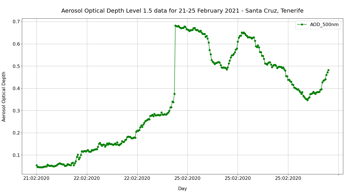
We can now plot the column AOD_500nm as time-series. What is striking in the resulting plot?
# Initiate a matplotlib figure
fig = plt.figure(figsize=(20,10))
ax=plt.axes()

# Select pandas dataframe columns and define a line plot
df.filter(['AOD_500nm']).plot(ax=ax, style='o-', color='green' )


# Set title and axes lable information
plt.title('\nAerosol Optical Depth Level 1.5 data for 21-25 February 2021 - Santa Cruz, Tenerife', fontsize=20, pad=20)
plt.ylabel('Aerosol Optical Depth\n', fontsize=16)
plt.xlabel('\nDay', fontsize=16)

# Format the axes ticks
plt.xticks(fontsize=16)
plt.yticks(fontsize=16)

# Add additionally a legend and grid to the plot
plt.legend(fontsize=16,loc=0)
plt.grid()
3. Resample AERONET data to a 3-hourly resolution#
Above you see that it seems we do not have observations for 23rd and 24th February 2020 for the Santa Cruz station in Tenerife. A closer inspection of the index entry confirms that we only have measurements for 21st, 22nd and 25th.
df.index.values
array(['21:02:2020', '21:02:2020', '21:02:2020', '21:02:2020',
       '21:02:2020', '21:02:2020', '21:02:2020', '21:02:2020',
       '21:02:2020', '21:02:2020', '21:02:2020', '21:02:2020',
       '21:02:2020', '21:02:2020', '21:02:2020', '21:02:2020',
       '21:02:2020', '21:02:2020', '21:02:2020', '21:02:2020',
       '21:02:2020', '21:02:2020', '21:02:2020', '21:02:2020',
       '21:02:2020', '21:02:2020', '21:02:2020', '21:02:2020',
       '21:02:2020', '21:02:2020', '21:02:2020', '21:02:2020',
       '21:02:2020', '21:02:2020', '21:02:2020', '21:02:2020',
       '21:02:2020', '21:02:2020', '21:02:2020', '21:02:2020',
       '21:02:2020', '21:02:2020', '21:02:2020', '21:02:2020',
       '21:02:2020', '22:02:2020', '22:02:2020', '22:02:2020',
       '22:02:2020', '22:02:2020', '22:02:2020', '22:02:2020',
       '22:02:2020', '22:02:2020', '22:02:2020', '22:02:2020',
       '22:02:2020', '22:02:2020', '22:02:2020', '22:02:2020',
       '22:02:2020', '22:02:2020', '22:02:2020', '22:02:2020',
       '22:02:2020', '22:02:2020', '22:02:2020', '22:02:2020',
       '22:02:2020', '22:02:2020', '22:02:2020', '22:02:2020',
       '22:02:2020', '22:02:2020', '22:02:2020', '22:02:2020',
       '22:02:2020', '22:02:2020', '22:02:2020', '22:02:2020',
       '22:02:2020', '22:02:2020', '22:02:2020', '22:02:2020',
       '22:02:2020', '22:02:2020', '22:02:2020', '22:02:2020',
       '22:02:2020', '22:02:2020', '22:02:2020', '22:02:2020',
       '22:02:2020', '22:02:2020', '22:02:2020', '22:02:2020',
       '22:02:2020', '22:02:2020', '22:02:2020', '22:02:2020',
       '22:02:2020', '22:02:2020', '22:02:2020', '22:02:2020',
       '22:02:2020', '22:02:2020', '22:02:2020', '22:02:2020',
       '22:02:2020', '22:02:2020', '22:02:2020', '22:02:2020',
       '22:02:2020', '22:02:2020', '22:02:2020', '22:02:2020',
       '22:02:2020', '22:02:2020', '22:02:2020', '22:02:2020',
       '22:02:2020', '22:02:2020', '22:02:2020', '22:02:2020',
       '22:02:2020', '22:02:2020', '22:02:2020', '22:02:2020',
       '22:02:2020', '22:02:2020', '22:02:2020', '22:02:2020',
       '22:02:2020', '22:02:2020', '22:02:2020', '22:02:2020',
       '22:02:2020', '22:02:2020', '25:02:2020', '25:02:2020',
       '25:02:2020', '25:02:2020', '25:02:2020', '25:02:2020',
       '25:02:2020', '25:02:2020', '25:02:2020', '25:02:2020',
       '25:02:2020', '25:02:2020', '25:02:2020', '25:02:2020',
       '25:02:2020', '25:02:2020', '25:02:2020', '25:02:2020',
       '25:02:2020', '25:02:2020', '25:02:2020', '25:02:2020',
       '25:02:2020', '25:02:2020', '25:02:2020', '25:02:2020',
       '25:02:2020', '25:02:2020', '25:02:2020', '25:02:2020',
       '25:02:2020', '25:02:2020', '25:02:2020', '25:02:2020',
       '25:02:2020', '25:02:2020', '25:02:2020', '25:02:2020',
       '25:02:2020', '25:02:2020', '25:02:2020', '25:02:2020',
       '25:02:2020', '25:02:2020', '25:02:2020', '25:02:2020',
       '25:02:2020', '25:02:2020', '25:02:2020', '25:02:2020',
       '25:02:2020', '25:02:2020', '25:02:2020', '25:02:2020',
       '25:02:2020', '25:02:2020', '25:02:2020', '25:02:2020',
       '25:02:2020', '25:02:2020', '25:02:2020', '25:02:2020',
       '25:02:2020', '25:02:2020', '25:02:2020', '25:02:2020',
       '25:02:2020', '25:02:2020', '25:02:2020', '25:02:2020',
       '25:02:2020', '25:02:2020', '25:02:2020', '25:02:2020',
       '25:02:2020', '25:02:2020', '25:02:2020', '25:02:2020',
       '25:02:2020', '25:02:2020', '25:02:2020', '25:02:2020',
       '25:02:2020', '25:02:2020', '25:02:2020', '25:02:2020',
       '25:02:2020', '25:02:2020', '25:02:2020', '25:02:2020',
       '25:02:2020', '25:02:2020', '25:02:2020', '25:02:2020',
       '25:02:2020', '25:02:2020', '25:02:2020', '25:02:2020',
       '25:02:2020', '25:02:2020', '25:02:2020', '25:02:2020',
       '25:02:2020', '25:02:2020', '25:02:2020', '25:02:2020',
       '25:02:2020', '25:02:2020', '25:02:2020', '25:02:2020',
       '25:02:2020', '25:02:2020', '25:02:2020', '25:02:2020',
       '25:02:2020', '25:02:2020', '25:02:2020', '25:02:2020',
       '25:02:2020', '25:02:2020', '25:02:2020', '25:02:2020',
       '25:02:2020', '25:02:2020', '25:02:2020', '25:02:2020',
       '25:02:2020', '25:02:2020', '25:02:2020', '25:02:2020',
       '25:02:2020', '25:02:2020', '25:02:2020', '25:02:2020',
       '25:02:2020', '25:02:2020', '25:02:2020', '25:02:2020',
       '25:02:2020', '25:02:2020', '25:02:2020', '25:02:2020',
       '25:02:2020', '25:02:2020', '25:02:2020', '25:02:2020',
       '25:02:2020', '25:02:2020', '25:02:2020', '25:02:2020',
       '25:02:2020', '25:02:2020', '25:02:2020'], dtype=object)
From the dataframe above, let us only select the columns of interest for us. This makes the handling of the dataframe much easier. The columns of interest are: Time(hh:mm:ss) and AOD_500nm and you can use the function filter() to select specific columns.
aeronet_ts = df.filter(['Time(hh:mm:ss)','AOD_500nm'])
aeronet_ts
| Time(hh:mm:ss) | AOD_500nm | |
|---|---|---|
| Date(dd:mm:yyyy) | ||
| 21:02:2020 | 08:22:46 | 0.053515 |
| 21:02:2020 | 08:25:22 | 0.046500 |
| 21:02:2020 | 08:28:46 | 0.045808 |
| 21:02:2020 | 08:30:39 | 0.045296 |
| 21:02:2020 | 08:33:09 | 0.045245 |
| ... | ... | ... |
| 25:02:2020 | 18:06:09 | 0.436686 |
| 25:02:2020 | 18:09:31 | 0.441193 |
| 25:02:2020 | 18:13:14 | 0.460659 |
| 25:02:2020 | 18:15:09 | 0.471839 |
| 25:02:2020 | 18:17:13 | 0.482647 |
291 rows × 2 columns
The next step is to create an index as DateTimeIndex. For this, we want to first combine the index entries (date) and time stamp entries of the column Time(hh:mm:ss). We can do this simply by redefining the data frame’s index and combining both with adding the two columns together as a string.
In a second step, we then convert the newly created index entry to a DateTimeIndex format with the function to_datetime(). Important here, you have to specify the format of combined index string.
aeronet_ts.index = aeronet_ts.index + ' ' + aeronet_ts['Time(hh:mm:ss)']
aeronet_ts.index = pd.to_datetime(aeronet_ts.index, format = '%d:%m:%Y %H:%M:%S')
aeronet_ts
| Time(hh:mm:ss) | AOD_500nm | |
|---|---|---|
| 2020-02-21 08:22:46 | 08:22:46 | 0.053515 |
| 2020-02-21 08:25:22 | 08:25:22 | 0.046500 |
| 2020-02-21 08:28:46 | 08:28:46 | 0.045808 |
| 2020-02-21 08:30:39 | 08:30:39 | 0.045296 |
| 2020-02-21 08:33:09 | 08:33:09 | 0.045245 |
| ... | ... | ... |
| 2020-02-25 18:06:09 | 18:06:09 | 0.436686 |
| 2020-02-25 18:09:31 | 18:09:31 | 0.441193 |
| 2020-02-25 18:13:14 | 18:13:14 | 0.460659 |
| 2020-02-25 18:15:09 | 18:15:09 | 0.471839 |
| 2020-02-25 18:17:13 | 18:17:13 | 0.482647 |
291 rows × 2 columns
The MONARCH model has a three hourly resolution. For this reason, we have to adjust the temporal resolution of the AERONET observations and resample the data frame to a three hourly temporal resolution. Below, we use the function resample() and create the average of every 3-hours. The resulting dataframe has 37 row entries.
aeronet_ts_resample = aeronet_ts.resample('3H').mean()
aeronet_ts_resample
| AOD_500nm | |
|---|---|
| 2020-02-21 06:00:00 | 0.047250 |
| 2020-02-21 09:00:00 | 0.054734 |
| 2020-02-21 12:00:00 | 0.061003 |
| 2020-02-21 15:00:00 | 0.092615 |
| 2020-02-21 18:00:00 | NaN |
| 2020-02-21 21:00:00 | NaN |
| 2020-02-22 00:00:00 | NaN |
| 2020-02-22 03:00:00 | NaN |
| 2020-02-22 06:00:00 | 0.117495 |
| 2020-02-22 09:00:00 | 0.147488 |
| 2020-02-22 12:00:00 | 0.253696 |
| 2020-02-22 15:00:00 | 0.375537 |
| 2020-02-22 18:00:00 | NaN |
| 2020-02-22 21:00:00 | NaN |
| 2020-02-23 00:00:00 | NaN |
| 2020-02-23 03:00:00 | NaN |
| 2020-02-23 06:00:00 | NaN |
| 2020-02-23 09:00:00 | NaN |
| 2020-02-23 12:00:00 | NaN |
| 2020-02-23 15:00:00 | NaN |
| 2020-02-23 18:00:00 | NaN |
| 2020-02-23 21:00:00 | NaN |
| 2020-02-24 00:00:00 | NaN |
| 2020-02-24 03:00:00 | NaN |
| 2020-02-24 06:00:00 | NaN |
| 2020-02-24 09:00:00 | NaN |
| 2020-02-24 12:00:00 | NaN |
| 2020-02-24 15:00:00 | NaN |
| 2020-02-24 18:00:00 | NaN |
| 2020-02-24 21:00:00 | NaN |
| 2020-02-25 00:00:00 | NaN |
| 2020-02-25 03:00:00 | NaN |
| 2020-02-25 06:00:00 | 0.674464 |
| 2020-02-25 09:00:00 | 0.581988 |
| 2020-02-25 12:00:00 | 0.572472 |
| 2020-02-25 15:00:00 | 0.407499 |
| 2020-02-25 18:00:00 | 0.450671 |
4. Load time series of the forecasts from CAMS and the MONARCH model#
We can now load the time-series information of the CAMS and the MONARCH model forecasts for Santa Cruz, Tenerife. The time-series has been saved as csv file from yesterday’s assignment (see here).
The time-series is available under ../data/sdswas_ts.csv and can be loaded as pandas.DataFrame with the function read_csv().
The next step is then to convert the index of the loaded dataframe into a DateTimeIndex format, as this allows us to combine the different time-series.
sdswas_ts = pd.read_csv('../../eodata/case_study/sdswas_ts.csv')
sdswas_ts.index = sdswas_ts['time']
sdswas_ts.index = pd.to_datetime(sdswas_ts.index, format = '%Y-%m-%d %H:%M:%S')
sdswas_ts
| time | lon | lat | od550_dust | |
|---|---|---|---|---|
| time | ||||
| 2020-02-21 12:00:00 | 2020-02-21 12:00:00 | -16.333335 | 28.33333 | 0.000058 |
| 2020-02-21 15:00:00 | 2020-02-21 15:00:00 | -16.333335 | 28.33333 | 0.000019 |
| 2020-02-21 18:00:00 | 2020-02-21 18:00:00 | -16.333335 | 28.33333 | 0.000027 |
| 2020-02-21 21:00:00 | 2020-02-21 21:00:00 | -16.333335 | 28.33333 | 0.000207 |
| 2020-02-22 00:00:00 | 2020-02-22 00:00:00 | -16.333335 | 28.33333 | 0.000890 |
| 2020-02-22 03:00:00 | 2020-02-22 03:00:00 | -16.333335 | 28.33333 | 0.001751 |
| 2020-02-22 06:00:00 | 2020-02-22 06:00:00 | -16.333335 | 28.33333 | 0.009111 |
| 2020-02-22 09:00:00 | 2020-02-22 09:00:00 | -16.333335 | 28.33333 | 0.050932 |
| 2020-02-22 12:00:00 | 2020-02-22 12:00:00 | -16.333335 | 28.33333 | 0.203418 |
| 2020-02-22 15:00:00 | 2020-02-22 15:00:00 | -16.333335 | 28.33333 | 0.363704 |
| 2020-02-22 18:00:00 | 2020-02-22 18:00:00 | -16.333335 | 28.33333 | 0.433835 |
| 2020-02-22 21:00:00 | 2020-02-22 21:00:00 | -16.333335 | 28.33333 | 1.095499 |
| 2020-02-23 00:00:00 | 2020-02-23 00:00:00 | -16.333335 | 28.33333 | 2.165373 |
| 2020-02-23 03:00:00 | 2020-02-23 03:00:00 | -16.333335 | 28.33333 | 2.052836 |
| 2020-02-23 06:00:00 | 2020-02-23 06:00:00 | -16.333335 | 28.33333 | 0.861120 |
| 2020-02-23 09:00:00 | 2020-02-23 09:00:00 | -16.333335 | 28.33333 | 0.753394 |
| 2020-02-23 12:00:00 | 2020-02-23 12:00:00 | -16.333335 | 28.33333 | 0.466931 |
| 2020-02-23 15:00:00 | 2020-02-23 15:00:00 | -16.333335 | 28.33333 | 0.354274 |
| 2020-02-23 18:00:00 | 2020-02-23 18:00:00 | -16.333335 | 28.33333 | 0.320627 |
| 2020-02-23 21:00:00 | 2020-02-23 21:00:00 | -16.333335 | 28.33333 | 0.231225 |
| 2020-02-24 00:00:00 | 2020-02-24 00:00:00 | -16.333335 | 28.33333 | 0.179565 |
| 2020-02-24 03:00:00 | 2020-02-24 03:00:00 | -16.333335 | 28.33333 | 0.221447 |
| 2020-02-24 06:00:00 | 2020-02-24 06:00:00 | -16.333335 | 28.33333 | 0.477572 |
| 2020-02-24 09:00:00 | 2020-02-24 09:00:00 | -16.333335 | 28.33333 | 0.700524 |
| 2020-02-24 12:00:00 | 2020-02-24 12:00:00 | -16.333335 | 28.33333 | 1.151539 |
We repeat the same process for the time-series of the CAMS forecasts. We first read the csv file under ../data/cams_ts.csv with the function read_csv(). Then, we convert the index into a DateTimeIndex format.
cams_ts = pd.read_csv('../../eodata/case_study/cams_ts.csv')
cams_ts.index = cams_ts['time']
cams_ts.index = pd.to_datetime(cams_ts.index, format='%Y-%m-%d %H:%M:%S')
cams_ts
| time | longitude | latitude | duaod550 | |
|---|---|---|---|---|
| time | ||||
| 2020-02-21 12:00:00 | 2020-02-21 12:00:00 | -16.4 | 28.6 | 0.000568 |
| 2020-02-21 15:00:00 | 2020-02-21 15:00:00 | -16.4 | 28.6 | 0.000568 |
| 2020-02-21 18:00:00 | 2020-02-21 18:00:00 | -16.4 | 28.6 | 0.001460 |
| 2020-02-21 21:00:00 | 2020-02-21 21:00:00 | -16.4 | 28.6 | 0.002422 |
| 2020-02-22 00:00:00 | 2020-02-22 00:00:00 | -16.4 | 28.6 | 0.005306 |
| 2020-02-22 03:00:00 | 2020-02-22 03:00:00 | -16.4 | 28.6 | 0.011280 |
| 2020-02-22 06:00:00 | 2020-02-22 06:00:00 | -16.4 | 28.6 | 0.080772 |
| 2020-02-22 09:00:00 | 2020-02-22 09:00:00 | -16.4 | 28.6 | 0.203139 |
| 2020-02-22 12:00:00 | 2020-02-22 12:00:00 | -16.4 | 28.6 | 0.335806 |
| 2020-02-22 15:00:00 | 2020-02-22 15:00:00 | -16.4 | 28.6 | 0.501777 |
| 2020-02-22 18:00:00 | 2020-02-22 18:00:00 | -16.4 | 28.6 | 0.581158 |
| 2020-02-22 21:00:00 | 2020-02-22 21:00:00 | -16.4 | 28.6 | 0.755507 |
| 2020-02-23 00:00:00 | 2020-02-23 00:00:00 | -16.4 | 28.6 | 1.102213 |
| 2020-02-23 03:00:00 | 2020-02-23 03:00:00 | -16.4 | 28.6 | 1.210434 |
| 2020-02-23 06:00:00 | 2020-02-23 06:00:00 | -16.4 | 28.6 | 1.024824 |
| 2020-02-23 09:00:00 | 2020-02-23 09:00:00 | -16.4 | 28.6 | 0.905959 |
| 2020-02-23 12:00:00 | 2020-02-23 12:00:00 | -16.4 | 28.6 | 0.777000 |
| 2020-02-23 15:00:00 | 2020-02-23 15:00:00 | -16.4 | 28.6 | 0.603338 |
| 2020-02-23 18:00:00 | 2020-02-23 18:00:00 | -16.4 | 28.6 | 0.545107 |
| 2020-02-23 21:00:00 | 2020-02-23 21:00:00 | -16.4 | 28.6 | 0.492370 |
| 2020-02-24 00:00:00 | 2020-02-24 00:00:00 | -16.4 | 28.6 | 0.364715 |
| 2020-02-24 03:00:00 | 2020-02-24 03:00:00 | -16.4 | 28.6 | 0.281077 |
| 2020-02-24 06:00:00 | 2020-02-24 06:00:00 | -16.4 | 28.6 | 0.170247 |
| 2020-02-24 09:00:00 | 2020-02-24 09:00:00 | -16.4 | 28.6 | 0.219139 |
| 2020-02-24 12:00:00 | 2020-02-24 12:00:00 | -16.4 | 28.6 | 0.355102 |
| 2020-02-24 15:00:00 | 2020-02-24 15:00:00 | -16.4 | 28.6 | 0.515648 |
| 2020-02-24 18:00:00 | 2020-02-24 18:00:00 | -16.4 | 28.6 | 0.622153 |
| 2020-02-24 21:00:00 | 2020-02-24 21:00:00 | -16.4 | 28.6 | 0.886938 |
| 2020-02-25 00:00:00 | 2020-02-25 00:00:00 | -16.4 | 28.6 | 1.008824 |
| 2020-02-25 03:00:00 | 2020-02-25 03:00:00 | -16.4 | 28.6 | 0.765258 |
| 2020-02-25 06:00:00 | 2020-02-25 06:00:00 | -16.4 | 28.6 | 0.606290 |
5. Visually compare model forecasts with AERONET observations#
All the three time-series (aeronet_ts, sdswas_ts and cams_ts) have now the same temporal resolution. The DateTimeIndex format allows for an efficient handling of time-series information and also allows us to combine the three time-series into one pandas.DataFrame. We can use the function join() and combine the two data frames aeronet_ts and sdswas_ts. We can repeat the process to join the third column from the cams_ts.
The resulting dataframe has 37 row entries and three columns.
df_merged = aeronet_ts_resample.join(sdswas_ts['od550_dust'])
df_merged = df_merged.join(cams_ts['duaod550'])
df_merged
| AOD_500nm | od550_dust | duaod550 | |
|---|---|---|---|
| 2020-02-21 06:00:00 | 0.047250 | NaN | NaN |
| 2020-02-21 09:00:00 | 0.054734 | NaN | NaN |
| 2020-02-21 12:00:00 | 0.061003 | 0.000058 | 0.000568 |
| 2020-02-21 15:00:00 | 0.092615 | 0.000019 | 0.000568 |
| 2020-02-21 18:00:00 | NaN | 0.000027 | 0.001460 |
| 2020-02-21 21:00:00 | NaN | 0.000207 | 0.002422 |
| 2020-02-22 00:00:00 | NaN | 0.000890 | 0.005306 |
| 2020-02-22 03:00:00 | NaN | 0.001751 | 0.011280 |
| 2020-02-22 06:00:00 | 0.117495 | 0.009111 | 0.080772 |
| 2020-02-22 09:00:00 | 0.147488 | 0.050932 | 0.203139 |
| 2020-02-22 12:00:00 | 0.253696 | 0.203418 | 0.335806 |
| 2020-02-22 15:00:00 | 0.375537 | 0.363704 | 0.501777 |
| 2020-02-22 18:00:00 | NaN | 0.433835 | 0.581158 |
| 2020-02-22 21:00:00 | NaN | 1.095499 | 0.755507 |
| 2020-02-23 00:00:00 | NaN | 2.165373 | 1.102213 |
| 2020-02-23 03:00:00 | NaN | 2.052836 | 1.210434 |
| 2020-02-23 06:00:00 | NaN | 0.861120 | 1.024824 |
| 2020-02-23 09:00:00 | NaN | 0.753394 | 0.905959 |
| 2020-02-23 12:00:00 | NaN | 0.466931 | 0.777000 |
| 2020-02-23 15:00:00 | NaN | 0.354274 | 0.603338 |
| 2020-02-23 18:00:00 | NaN | 0.320627 | 0.545107 |
| 2020-02-23 21:00:00 | NaN | 0.231225 | 0.492370 |
| 2020-02-24 00:00:00 | NaN | 0.179565 | 0.364715 |
| 2020-02-24 03:00:00 | NaN | 0.221447 | 0.281077 |
| 2020-02-24 06:00:00 | NaN | 0.477572 | 0.170247 |
| 2020-02-24 09:00:00 | NaN | 0.700524 | 0.219139 |
| 2020-02-24 12:00:00 | NaN | 1.151539 | 0.355102 |
| 2020-02-24 15:00:00 | NaN | NaN | 0.515648 |
| 2020-02-24 18:00:00 | NaN | NaN | 0.622153 |
| 2020-02-24 21:00:00 | NaN | NaN | 0.886938 |
| 2020-02-25 00:00:00 | NaN | NaN | 1.008824 |
| 2020-02-25 03:00:00 | NaN | NaN | 0.765258 |
| 2020-02-25 06:00:00 | 0.674464 | NaN | 0.606290 |
| 2020-02-25 09:00:00 | 0.581988 | NaN | NaN |
| 2020-02-25 12:00:00 | 0.572472 | NaN | NaN |
| 2020-02-25 15:00:00 | 0.407499 | NaN | NaN |
| 2020-02-25 18:00:00 | 0.450671 | NaN | NaN |
The last step is now to plot the three columns of the pandas.DataFrame df_merged as three individual line plots.
# Initiate a figure
fig = plt.figure(figsize=(15,8))
ax = plt.subplot()

# Define the plotting function
ax.plot(df_merged.od550_dust, 'o-', color='darkred',  label='SDS-WAS dust forecast - 550 nm')
ax.plot(df_merged.duaod550, 'o-', color='blue', label='CAMS dust forecast - 550 nm')
ax.plot(df_merged.AOD_500nm, 'o-', color='green', label='AERONET observations - 500 nm')

# Customize the title and axes lables
ax.set_title('\nAerosol Optical Depth at 500 / 550 nm - Santa Cruz, Tenerife\n', fontsize=20)
ax.set_ylabel('~', fontsize=14)
ax.set_xlabel('\nHour', fontsize=14)

# Customize the fontsize of the axes tickes
plt.xticks(fontsize=14)
plt.yticks(fontsize=14)

# Add a gridline to the plot
ax.grid(linestyle='--')

plt.legend(fontsize=14, loc=2)
<matplotlib.legend.Legend at 0x7f12a26f02b0>
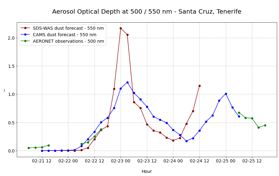
The plot above shows you that AERONET station observations can be used to evaluate model predictions - however, station observations show often also quite a few gaps. The strong dust event over Tenerife on 23/24 February 2021 was not measured at all by the AERONET station. For such gaps, model data are helpful to bridge such gaps. But the plot above shows also that the two models predicted especially the intensity of the dust event differently.