SDS-WAS regional dust forecasts

SDS-WAS regional dust forecasts#

Hint

Execute the notebook on the training platform >>

This notebook provides an introduction to dust forecast data from the MONARCH model. The notebook introduces you to the variable Dust Optical Depth and you will learn how the model has predicted the Saharan Dust event which occured over Europe in the first half of April 2024.

The WMO Sand and Dust Storm Warning Advisory and Assessment System (SDS-WAS). is an international framework linking institutions involved in Sand and Dust Storm (SDS) research, operations and delivery of services.

The framework is organised in several regional centers, which aim to implement SDS-WAS objectives in a specific region. The Barcelona Supercomputing Center (BSC-CNS) and the Meteorological State Agency of Spain (AEMET) are hosting the SDS-WAS regional center for Northern Africa, Middle East and Europe.

One of the main activities of the SDS-WAS regional center is to provide daily operational dust forecasts for Northern Africa (north of the equator), Middle East and Europe. The BCS-CNS, in collaboration with NOAA’s National Centers for Environmental Prediction (NCEP), the NASA’s Goddard Institute for Space Studies and the International Research Institute for Climate Society (IRI), has developed MONARCH, an online multi-scale atmospheric dust model intended to provide short and medium-range dust forecasts for both, regional and global domains.

The model provides forecast information up to 72 hours in advance (every 3 hours) of two parameters: Dust Optical Depth and Dust Surface Concentration.

MONARCH Forecast data are available in netCDF format and are available for download via a THREDDS Data Server here.

Basic facts

Spatial resolution: 0.1° x 0.1°
Spatial coverage: Northern Africa, Middle East and Europe
Temporal resolution: 3-hourly up to 72 hours in advance
Temporal coverage: since February 2012
Data format: NetCDF

How to access the data

Dust forecast data from the MONARCH model are available for download via the website of the WMO Barcelona Dust Regional Center.

In order to be able to download data from the portal, you need to register via this contact form. Below, you see an example how you can programmatically download one data file.

Learn more about the data products and how to access them from this user guide.

Load required libraries

import xarray as xr
import requests

import matplotlib.pyplot as plt
import matplotlib.colors
from matplotlib.cm import get_cmap
from matplotlib import animation
from matplotlib.axes import Axes

import cartopy.crs as ccrs
from cartopy.mpl.gridliner import LONGITUDE_FORMATTER, LATITUDE_FORMATTER
import cartopy.feature as cfeature
from cartopy.mpl.geoaxes import GeoAxes
GeoAxes._pcolormesh_patched = Axes.pcolormesh

from IPython.display import HTML

import warnings
warnings.simplefilter(action = "ignore", category = RuntimeWarning)

Load helper functions

%run ../functions.ipynb

Download MONARCH dust forecast data#

Data products from the WMO Barcelona Dust Regional Center can be accessed via a THREDDS Data Server. After registration, you received access credentials that you can use to access the data files. You can store your access credentials as variables, user and password respectively. Note: you have to replace the ##### with your credentials.

user='################'
password='###################'

The data catalog offers public and restricted data. MONARCH dust forecasts are available as public data files. To get the download link for the dust forecast issued on 7 April 2024, you have to navigate to the following folder in the data catalog: /BDRC_THREDDS_Public_Data/MONARCH/2024/04/. If you click on the file for 7 April 2024, you get different download options. In the following, you see an example how you can use the Python library requests to download data from a given url.

First, let us store the url path of the data file as variable.

url='https://dust.aemet.es/thredds/fileServer/dataRoot/MONARCH/2024/04/2024040712_3H_SDSWAS_NMMB-BSC-v2_OPER.nc'

Next, you can now establish a connection to the server where the data file is hosted, with the function get() from the requests package. You have to specify auth as keyword argument and give the function your access credentials (user, password).

Once a successful connection is established, you can open a new file and write the content of the server connection. The result is a netCDF data with a size of ~900 MB.

r = requests.get(url, auth=(user,password))
open('./20240407_MONARCH_dust_forecast.nc', 'wb').write(r.content)

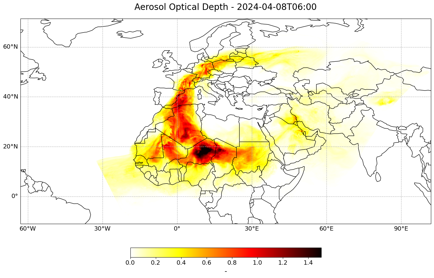
Visualize dust AOD at 550 nm#

Now we have loaded all necessary information to be able to visualize the dust Aerosol Optical Depth for one specific time during the forecast run. Let us use the function visualize_pcolormesh() to visualize the data with the help of the plotting library matplotlib and Cartopy.

You have to specify the following keyword arguments:

data_array: the
longitude, latitude: longitude and latitude variables of the data variable
projection: one of Cartopy’s projection options
color_scale: one of matplotlib’s colormaps
units: unit of the data parameter, preferably taken from the data array’s attributes
long_name: longname of the data parameter is taken as title of the plot, preferably taken from the data array’s attributes
vmin, vmax: minimum and maximum bounds of the color range
set_global: False, if data is not global
lonmin, lonmax, latmin, latmax: kwargs have to be specified, if set_global=False

Note: in order to have the time information as part of the title, we add the string of the datetime information to the long_name variable: long_name + ' ' + str(od_dust[##,:,:].time.data)[0:16].

forecast_step = 6
visualize_pcolormesh(data_array=od_dust[forecast_step,:,:],
                     longitude=od_dust.lon,
                     latitude=od_dust.lat,
                     projection=ccrs.PlateCarree(),
                     color_scale='hot_r',
                     unit=units,
                     long_name='Aerosol Optical Depth - ' + str(od_dust[forecast_step,:,:].time.data)[0:16],
                     vmin=0, 
                     vmax=1.5,
                     set_global=False,
                     lonmin=longitude.min().data,
                     lonmax=longitude.max().data,
                     latmin=latitude.min().data,
                     latmax=latitude.max().data)

(<Figure size 2000x1000 with 2 Axes>,
 <GeoAxes: title={'center': 'Aerosol Optical Depth - 2024-04-08T06:00'}>)

../_images/72ed221b839a214bd705e5e8ea17903335f860fcc7b8111d878755de9b167710.png

Animate dust AOD forecasts#

In the last step, you can animate the Dust Aerosol Optical Depth forecasts in order to see how the trace gas develops over a period of 3 days, from 7th April 2024 12 UTC to 10th April 2024.

You can do animations with matplotlib’s function animation. Jupyter’s function HTML can then be used to display HTML and video content.

The animation function consists of 4 parts:

Setting the initial state:
Here, you define the general plot your animation shall use to initialise the animation. You can also define the number of frames (time steps) your animation shall have.
Functions to animate:
An animation consists of three functions: draw(), init() and animate(). draw() is the function where individual frames are passed on and the figure is returned as image. In this example, the function redraws the plot for each time step. init() returns the figure you defined for the initial state. animate() returns the draw() function and animates the function over the given number of frames (time steps).
Create a animate.FuncAnimation object:
The functions defined before are now combined to build an animate.FuncAnimation object.
Play the animation as video:
As a final step, you can integrate the animation into the notebook with the HTML class. You take the generate animation object and convert it to a HTML5 video with the to_html5_video function

# Setting the initial state:
# 1. Define figure for initial plot
fig, ax = visualize_pcolormesh(data_array=od_dust[0,:,:],
                     longitude=od_dust.lon,
                     latitude=od_dust.lat,
                     projection=ccrs.PlateCarree(),
                     color_scale='hot_r',
                     unit=units,
                     long_name='Aerosol Optical Depth - ' + str(od_dust[0,:,:].time.data)[0:16],
                     vmin=0, 
                     vmax=1.5,
                     lonmin=longitude.min().data,
                     lonmax=longitude.max().data,
                     latmin=latitude.min().data,
                     latmax=latitude.max().data,
                     set_global=False)

frames = 24

def draw(i):
    img = plt.pcolormesh(od_dust.lon, 
                         od_dust.lat, 
                         od_dust[i,:,:], 
                         cmap='hot_r', 
                         transform=ccrs.PlateCarree(),
                         vmin=0,
                         vmax=1.5,
                         shading='auto')
    
    ax.set_title('Aerosol Optical Depth - '+ str(od_dust.time[i].data)[0:16], fontsize=20, pad=20.0)
    return img


def init():
    return fig


def animate(i):
    return draw(i)

ani = animation.FuncAnimation(fig, animate, frames, interval=800, blit=False,
                              init_func=init, repeat=True)

HTML(ani.to_html5_video())
plt.close(fig)

HTML(ani.to_html5_video())

SDS-WAS regional dust forecasts

Contents

SDS-WAS regional dust forecasts#

Download MONARCH dust forecast data#

Load and browse MONARCH dust forecast data#

Load data variables as data arrays#

Visualize dust AOD at 550 nm#

Animate dust AOD forecasts#