.ipynb .pdf

Contents

MSG SEVIRI RGB composites

Hint

Execute the notebook on the training platform >>

This notebook provides you an introduction to Level 1.5 data from the SEVIRI instrument as part of the Meteosat Second Generation 0 Degree Service. It further provides you an introduction to the Python package satpy which allows for an efficient handling of data from meteorological satellite instruments, including SEVIRI and MODIS. At the end, a specific focus will be put on the SEVIRI Dust RGB, whose primary aim is to detect dust in the atmosphere.

The example features the saharan dust event during 5./6. February 2021, which brought massive amounts of Saharan dust into central Europe. See a more detailed description of this particular event here.

The Meteosat series have been providing crucial data for weather forecasting since 1977 and is a series of geostationary satellites providing imagery for weather forecasting and climate monitoring. Meteosat Second Genersation (MSG) is the current fleet of operational geostationary satellites. The Spinning Enhanced Visible and InfraRed Imager (SEVIRI) is MSG’s primary instrument and has the capacity to observe the Earth in 12 spectral channels. 11 channels provides measurements with a resolution of 3 km at the sub-satellite and one, the High Resolution Visible (HRV) channel, provides measurements with a resolution of 1 km.

The SEVIRI instrument allows for a complete image scan (Full Earth Scan) every 15 minutes. The 0 Degree Service is the main mission of MSG and provides High Rate SEVIRI image data in 12 spectral bands, processed in near real-time to Level 1.5.

Basic facts

Spatial resolution: 1 km at nadir
Spatial coverage: Latitude: -81 to 81 degrees, Longitude: -79 to 79 degrees
Revisit time: every 15 minutes
Data availability: since 2004

How to access the data

High Rate SEVIRI Level 1.5 Image Data is available for download via the EUMETSAT Data Store. You need to register for the EUMETSAT Earth Observation Portal in order to be able to download data from the Data Store.

---

Load required libraries

import glob
import xarray as xr
import numpy as np

import matplotlib.pyplot as plt
import matplotlib.colors
from matplotlib.axes import Axes

import cartopy
import cartopy.crs as ccrs
from cartopy.mpl.gridliner import LONGITUDE_FORMATTER, LATITUDE_FORMATTER
from cartopy.mpl.geoaxes import GeoAxes
GeoAxes._pcolormesh_patched = Axes.pcolormesh

from satpy.scene import Scene
from satpy.composites import GenericCompositor
from satpy.writers import to_image
from satpy.resample import get_area_def
from satpy import available_readers

import pyresample

import warnings
warnings.filterwarnings('ignore')
warnings.simplefilter(action = "ignore", category = RuntimeWarning)

Load helper functions

%run ../../functions.ipynb

---

MSG SEVIRI True color composite

Load and browse High Rate SEVIRI Level 1.5 image data

Meteosat Second Generation data are disseminated in the specific MSG Level 1.5 Native format. The Python package satpy supports reading and loading data from many input files. With the function available_readers(), you can get a list of all available readers satpy offers. For MSG data and the Native format, you can use the reader seviri_l1b_native.

available_readers()

From the EUMETSAT Data Store, we downloaded for severals hours from 5./6. February 2021 of High Rate SEVIRI Level 1.5 Image data. The data is available in the folder ../../eodata/1_satellite/meteosat/event/. Let us load one image scence for 6 February at 7.27 UTC. First, we specify the file path and create a variable with the name file_name.

file_name = glob.glob('../../eodata/1_satellite/meteosat/event/*2021020607*.nat')
file_name

In a next step, we use the Scene constructor from the satpy library. Once loaded, a Scene object represents a single geographic region of data, typically at a single continuous time range.

You have to specify the two keyword arguments reader and filenames in order to successfully load a scene. As mentioned above, for MSG SEVIRI data in the Native format, you can use the seviri_l1b_native reader.

scn = Scene(reader="seviri_l1b_native", 
             filenames=file_name)
scn

<satpy.scene.Scene at 0x7fdb8f7cda90>

A Scene object loads all band information of a satellite image. With the function available_dataset_names(), you can see the available bands available from the MSG SEVIRI satellite.

scn.available_dataset_names()

['HRV',
 'IR_016',
 'IR_039',
 'IR_087',
 'IR_097',
 'IR_108',
 'IR_120',
 'IR_134',
 'VIS006',
 'VIS008',
 'WV_062',
 'WV_073']

The underlying container for data in satpy is the xarray.DataArray. With the function load(), you can specify an individual band by name, e.g. IR_108 and load the data. If you then select the loaded band, you see that the band object is a xarray.DataArray.

scn.load(['IR_108'])
scn['IR_108']

<xarray.DataArray 'reshape-7f46b2a2eee50e746a278c951ee5cd2d' (y: 3712, x: 3712)>
dask.array<truediv, shape=(3712, 3712), dtype=float32, chunksize=(3712, 3712), chunktype=numpy.ndarray>
Coordinates:
    acq_time  (y) datetime64[ns] NaT NaT NaT NaT NaT NaT ... NaT NaT NaT NaT NaT
    crs       object PROJCRS["unknown",BASEGEOGCRS["unknown",DATUM["unknown",...
  * y         (y) float64 -5.566e+06 -5.563e+06 ... 5.566e+06 5.569e+06
  * x         (x) float64 5.566e+06 5.563e+06 5.56e+06 ... -5.566e+06 -5.569e+06
Attributes: (12/17)
    orbital_parameters:       {'projection_longitude': 0.0, 'projection_latit...
    units:                    K
    wavelength:               10.8 µm (9.8-11.8 µm)
    standard_name:            toa_brightness_temperature
    platform_name:            Meteosat-11
    sensor:                   seviri
    ...                       ...
    name:                     IR_108
    resolution:               3000.403165817
    calibration:              brightness_temperature
    modifiers:                ()
    _satpy_id:                DataID(name='IR_108', wavelength=WavelengthRang...
    ancillary_variables:      []

With an xarray data structure, you can handle the object as a xarray.DataArray. For example, you can print a list of available attributes with the function attrs.keys().

scn['IR_108'].attrs.keys()

dict_keys(['orbital_parameters', 'units', 'wavelength', 'standard_name', 'platform_name', 'sensor', 'georef_offset_corrected', 'start_time', 'end_time', 'reader', 'area', 'name', 'resolution', 'calibration', 'modifiers', '_satpy_id', 'ancillary_variables'])

With the attrs() function, you can also access individual metadata information, e.g. start_time and end_time.

scn['IR_108'].attrs['start_time'], scn['IR_108'].attrs['end_time']

(datetime.datetime(2021, 2, 6, 7, 15, 11, 201331),
 datetime.datetime(2021, 2, 6, 7, 30, 10, 197941))

But for now, let us reload the data file from the beginning. We do not need the IR_108 channel for the next steps, but rather would like to focus on different RGB composites.

scn = Scene(reader="seviri_l1b_native", 
             filenames=file_name)
scn

<satpy.scene.Scene at 0x7f05fb7933a0>

Browse and visualize RGB composite IDs

RGB composites combine multiple window channels of satellite data in order to get e.g. a true-color image of the scene. Depending on the channel combination used, different features can be highlighted in the composite, e.g. dust. SatPy offers several predefined RGB composites options. The function available_composite_ids() returns a list of available composite IDs. You see that there are predefined composites for e.g. natural_color, snow or dust.

scn.available_composite_ids()

[DataID(name='airmass'),
 DataID(name='ash'),
 DataID(name='cloudtop'),
 DataID(name='cloudtop_daytime'),
 DataID(name='colorized_ir_clouds'),
 DataID(name='convection'),
 DataID(name='day_microphysics'),
 DataID(name='day_microphysics_winter'),
 DataID(name='dust'),
 DataID(name='fog'),
 DataID(name='green_snow'),
 DataID(name='hrv_clouds'),
 DataID(name='hrv_fog'),
 DataID(name='hrv_severe_storms'),
 DataID(name='hrv_severe_storms_masked'),
 DataID(name='ir108_3d'),
 DataID(name='ir_cloud_day'),
 DataID(name='ir_overview'),
 DataID(name='ir_sandwich'),
 DataID(name='natural_color'),
 DataID(name='natural_color_nocorr'),
 DataID(name='natural_color_raw'),
 DataID(name='natural_color_with_night_ir'),
 DataID(name='natural_color_with_night_ir_hires'),
 DataID(name='natural_enh'),
 DataID(name='natural_enh_with_night_ir'),
 DataID(name='natural_enh_with_night_ir_hires'),
 DataID(name='natural_with_night_fog'),
 DataID(name='night_fog'),
 DataID(name='night_ir_alpha'),
 DataID(name='night_ir_with_background'),
 DataID(name='night_ir_with_background_hires'),
 DataID(name='night_microphysics'),
 DataID(name='overview'),
 DataID(name='overview_raw'),
 DataID(name='realistic_colors'),
 DataID(name='snow'),
 DataID(name='vis_sharpened_ir')]

Let us define a list with the composite ID natural_color. This list (composite_id) can then be passed to the function load(). Per default, scenes are loaded with the north pole facing downwards. You can specify the keyword argument upper_right_corner="NE" in order to turn the image around and have the north pole facing upwards.

composite_id = ['natural_color']
scn.load(composite_id, upper_right_corner="NE")

A print of the Scene object scn shows you that it consists of one xarray.DataArray with the standard name natural_color.

print(scn)

<xarray.DataArray 'where-c726622c80224770c3c041125613789c' (bands: 3, y: 3712, x: 3712)>
dask.array<where, shape=(3, 3712, 3712), dtype=float64, chunksize=(1, 3712, 3712), chunktype=numpy.ndarray>
Coordinates:
    crs      object PROJCRS["unknown",BASEGEOGCRS["unknown",DATUM["unknown",E...
  * y        (y) float64 5.569e+06 5.566e+06 5.563e+06 ... -5.563e+06 -5.566e+06
  * x        (x) float64 -5.569e+06 -5.566e+06 ... 5.563e+06 5.566e+06
  * bands    (bands) <U1 'R' 'G' 'B'
Attributes: (12/20)
    georef_offset_corrected:                True
    area:                                   Area ID: msg_seviri_fes_3km\nDesc...
    end_time:                               2021-02-06 07:30:10.197941
    platform_name:                          Meteosat-11
    sun_earth_distance_correction_applied:  True
    reader:                                 seviri_l1b_native
    ...                                     ...
    optional_datasets:                      []
    name:                                   natural_color
    _satpy_id:                              DataID(name='natural_color', reso...
    prerequisites:                          [DataQuery(name='IR_016', modifie...
    optional_prerequisites:                 []
    mode:                                   RGB

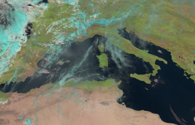
The function show() allows you to visualize a loaded composite or band. Let us e.g. visualize the natural_color composite. Once visualized, you see that the RGB composite highlights clouds in turquoise, but highlights specific features in their natural color.

scn.show('natural_color')

Generate a geographical subset for southern Europe

The visualization above looks nice, but in many cases you might want to highlight a specific geographical region. Let us generate a geographical subset for southern Europe. You can do this with the function crop() and specifying the keyword argument ll_bbox=(lon_min, lat_min, lon_max, lat_max). Let us take the following bounding box information with a focus over Portugal and Spain: (-5.0, 31.0, 20.0, 51.0).

Afterwards, you can visualize the cropped image with the function show().

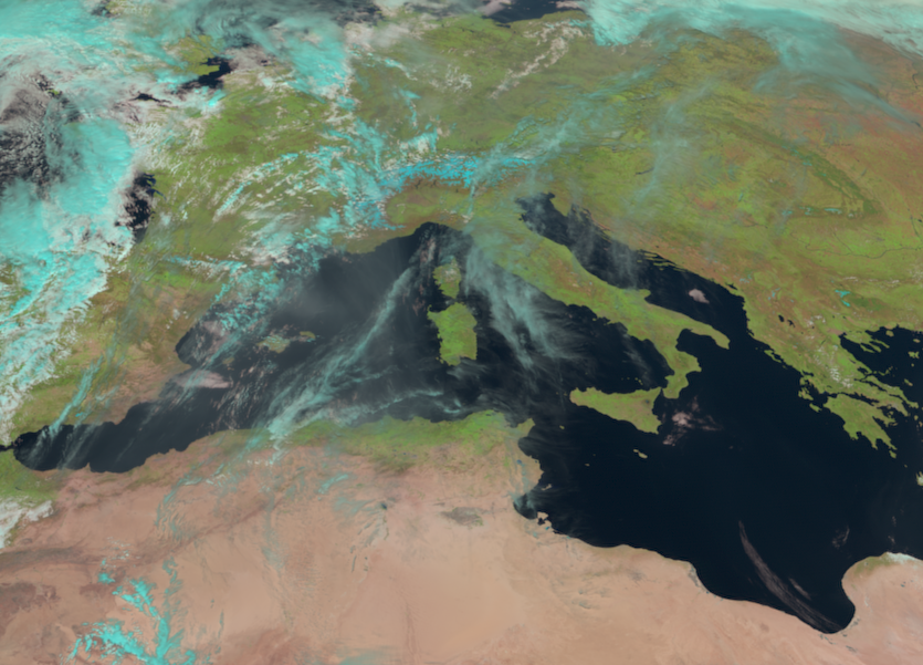
scn_cropped = scn.crop(ll_bbox=(-5, 31, 20, 51))
scn_cropped.show("natural_color")

From the cropped image, you can load the area information that is stored as an attribute entry. The area attribute holds information related to the projection, number of columns / rows and area extent.

Note: the area extent key provides x and y values in meters from the nadir, which is the original projection unit.

scn_cropped['natural_color'].attrs['area']

Area ID: msg_seviri_fes_3km
Description: MSG SEVIRI Full Earth Scanning service area definition with 3 km resolution
Projection: {'a': '6378169', 'h': '35785831', 'lon_0': '0', 'no_defs': 'None', 'proj': 'geos', 'rf': '295.488065897014', 'type': 'crs', 'units': 'm', 'x_0': '0', 'y_0': '0'}
Number of columns: 750
Number of rows: 482
Area extent: (-454561.0796, 3151923.5257, 1795741.2947, 4598117.8516)

Another possibility is to crop the data with x and y values in original projection unit (x_min, y_min, x_max, y_max). In the case of MSG SEVIRI data, the projection unit is meters (distance from the nadir). Below we apply the funcion crop() again, but instead of ll_bbox, we use this time the keyword argument xy_bbox=(xmin, ymin, xmax, ymax) and slightly adjust the x and y values from the area extent attribute above.

When we visualize the cropped image again with the function show(), you see that the extent is more or less the same. The adjustment of ymin and ymax has increased the extent towards the north and the south.

scn_cropped = scn.crop(xy_bbox=(-5E5, 30E5, 20E5, 48E5))
scn_cropped.show("natural_color")

As a next step, let us store the area definition as variable and call it area. We can can use the area information to resample the loaded scene object in a next step.

area = scn_cropped['natural_color'].attrs['area']
area

Area ID: msg_seviri_fes_3km
Description: MSG SEVIRI Full Earth Scanning service area definition with 3 km resolution
Projection: {'a': '6378169', 'h': '35785831', 'lon_0': '0', 'no_defs': 'None', 'proj': 'geos', 'rf': '295.488065897014', 'type': 'crs', 'units': 'm', 'x_0': '0', 'y_0': '0'}
Number of columns: 835
Number of rows: 601
Area extent: (-502567.5303, 2998902.9642, 2002769.1132, 4802145.2669)

Cropping is nice and for our geographical area of interest the cropped image looks acceptable. However, when working with regions close to the marging of the scene, the cropped scene can look very distorted, due to the viewing angle of the satellite. For this reason, it is recommended to use the function resample() from the library pyresample, which resamples the loaded scene to a custom area and projection.

Pyresample offers predefined areas; a list of those can be found in the satpy package under /satpy/etc/ in the file areas.yaml. There is no predefined area for our region. For this reason, we can make use of the variable area, which we defined above and which has all the area information needed by the resample() function. Below, we simply pass the area variable to the resample() function.

scn_resample_nc = scn.resample(area)
scn_resample_nc.show('natural_color')

Visualize MSG SEVIRI true color composite with Cartopy features

SatPy’s built-in visualization function is nice, but often you want to make use of additonal features, such as country borders. The library Cartopy offers powerful functions that enable the visualization of geospatial data in different projections and to add additional features to a plot. Below, we will show you how you can visualize the natural_color composite with the two Python packages matplotlib and Cartopy.

As a first step, we have to convert the Scene object into a numpy array. The numpy array additionally needs to be transposed to a shape that can be interpreted by matplotlib’s function imshow(): (M,N,3). You can convert a Scene object into a numpy.array object with the function np.asarray().

The shape of the array is (3, 601, 667). This means we have to transpose the array and add index=0 on index position 3.

image = np.asarray(scn_resample_nc["natural_color"]).transpose(1,2,0)
image.shape

(601, 835, 3)

In a next step, we scale the values to a range between 0 and 1 and we clip the lower and upper percentiles. This process sharpens the contrast, as a potential contrast decrease caused by outliers is eliminated.

image = np.interp(image, (np.percentile(image,1), np.percentile(image,99)), (0, 1))

Let us now also define a variable for the coordinate reference system. We take the area attribute from she scn_resample_nc Scene and convert it with the function to_cartopy_crs() into a format Cartopy can read. We will use the crs information for plotting.

crs = scn_resample_nc["natural_color"].attrs["area"].to_cartopy_crs()

Now, we can visualize the natural_color composite. The plotting code can be divided in four main parts:

• Initiate a matplotlib figure: Initiate a matplotlib plot and define the size of the plot

• Specify coastlines and a grid: specify additional features to be added to the plot

• Plotting function: plot the numpy array with the plotting function imshow()

• Set plot title: specify title of the plot

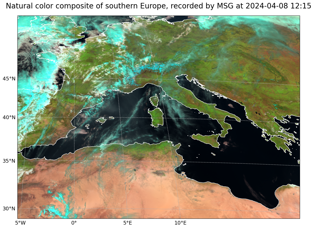
# Initiatie a subplot and axes with the CRS information previously defined
fig = plt.figure(figsize=(16, 10))
ax = fig.add_subplot(1, 1, 1, projection=crs)

# Add coastline features to the plot
ax.coastlines(resolution="10m", color="white")

# Define a grid to be added to the plot
gl = ax.gridlines(draw_labels=True, linestyle='--', xlocs=range(-10,11,5), ylocs=range(30,50,5))
gl.top_labels=False
gl.right_labels=False
gl.xformatter=LONGITUDE_FORMATTER
gl.yformatter=LATITUDE_FORMATTER
gl.xlabel_style={'size':14}
gl.ylabel_style={'size':14}

# In the end, we can plot our image data...
ax.imshow(image, transform=crs, extent=crs.bounds, origin="upper")

# Define a title for the plot
plt.title("Natural color composite of southern Europe, recorded by MSG at " + scn_resample_nc.attrs["start_time"].strftime("%Y-%m-%d %H:%M"), fontsize=20, pad=20.0)

Text(0.5, 1.0, 'Natural color composite of southern Europe, recorded by MSG at 2021-02-06 07:15')

MSG SEVIRI Dust RGB composite

In a final step, we would like to have a closer look at the SEVIRI Dust RGB composite, whose primary aim is to support the detection of dust in the atmosphere. The dust composite makes use of three window channels of Meteosat Second Generation:

• Red: IR12.0-IR10.8

• Green: IR10.8-IR.8.7

• Blue: IR10.8

Let us first again load the image from 6 February 2021 at 7.27 UTC as a pytroll Scene object again.

file_name = glob.glob('../../eodata/1_satellite/meteosat/event/*2021020607*.nat')
file_name

Now, let us define a list with the predefined dust RGB composite and let us load this composite with the function load(). Remember, by specifying the keyword argument upper_right_corner='NE', you load the image with North facing upwards.

composite_id = ['dust']
scn.load(composite_id, upper_right_corner="NE")

The, we can directly resample the image to the area defined above. You can use the area object and the function resample() to resample the dust RGB composite to the area of interest.

scn_resample_dust = scn.resample(area)

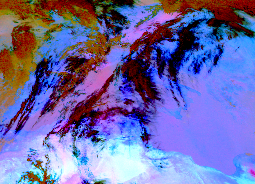
And in a last step, we can visualize the dust composite with Satpy’s built-in visualization function show(). The colours of the dust RGB can be interpreted as follows:

• Magenta: Dust or ash clouds

• Black: Cirrus clouds

• Dark red: Thick, high and cold ice clouds

• Yellow: Thick mid-level clouds

• Darkblue: Humid air in lower levels

• Lilac: Dry air in lower levels

Get more information about the Dust RGB in the SEVIRI Dust RGB Quick Guide.

The dust composite of 6 February at 7.27 UTC shows clearly a dust cloud below a thicker ice cloud over the northern mediterranean sea and the Alps. You also see that the dust cloud is coming from the Sahara towards Europe.

scn_resample_dust.show('dust')

References

• MSG 0-degree service

• SEVIRI Dust RGB - Quick Guide

• Meteosat-11 captures plume of Saharan dust

• Meteosat series

• Meteosat Second Generation

• SEVIRI Dust RGB Quick Guide

previous

Remote Sensing - Satellite

next

Terra/Aqua MODIS RGB composites