.ipynb .pdf

Contents

Terra/Aqua MODIS RGB composites

Hint

Execute the notebook on the training platform >>

This module shows the structure of MODIS MOD021K Level 1B Calibrated Radiances data and what information of the data files can be used in order to load, browse and visualize the data.

According to NASA, “The MODIS Level 1B data set contains calibrated and geolocated at-aperture radiances for 36 discrete bands located in the 0.4 µm to 14.4 µm region of the electromagentic spectrum. These data are generated from MODIS Level-1A scans of raw radiance, and in the process are converted to geophysical units of W/(m2 µm sr).”

Basic facts

Spatial resolution: 1 km at nadir
Spatial coverage: Global
Revisit time: Daily
Data availability: since 2002

How to access the data

This notebook uses the MODIS MOD21K dataset from the Terra platform. This data can be ordered via the LAADS DAAC and are distributed in HDF4-EOS format, which is based on HDF4. You need to register for an Earthdata account in order to be able to download data.

---

Load required libraries

import glob
import numpy as np

import matplotlib.pyplot as plt
import matplotlib.colors
from matplotlib.axes import Axes

import satpy
from satpy.scene import Scene
from satpy import find_files_and_readers
import pyresample as prs

import cartopy.crs as ccrs
from cartopy.mpl.gridliner import LONGITUDE_FORMATTER, LATITUDE_FORMATTER
from cartopy.mpl.geoaxes import GeoAxes
GeoAxes._pcolormesh_patched = Axes.pcolormesh

import warnings
warnings.filterwarnings('ignore')
warnings.simplefilter(action = "ignore", category = RuntimeWarning)

Load helper functions

%run ../../functions.ipynb

---

Load and browse MODIS Level 1B Calibrated Radiances data

MODIS data is disseminated in the HDF4-EOS format. We will use the Python library satpy to open the data. The results in a netCDF4.Dataset, which contains the dataset’s metadata, dimension and variable information.

Read more about satpy here.

From the LAADS DAAC, we downloaded one tile of Level-1B Image data on 6 February 2021. The data is available in the folder ../../eodata/1_satellite/modis/level_1b/2021/02/06/. Let us load the data. First, we specify the file path and create a variable with the name file_name.

file_name = glob.glob('../../eodata/1_satellite/modis/level_1b/2021/02/06/MOD021KM.A2021037.1015.061.2021038015551.hdf')
file_name

In a next step, we use the Scene constructor from the satpy library. Once loaded, a Scene object represents a single geographic region of data, typically at a single continuous time range.

You have to specify the two keyword arguments reader and filenames in order to successfully load a scene. As mentioned above, for MODIS Level-1B data, you can use the modis_l1b reader.

scn =Scene(filenames=file_name,reader='modis_l1b')

scn

<satpy.scene.Scene at 0x7f60180b4460>

A Scene object is a collection of different bands, with the function available_dataset_names(), you can see the available bands of the scene. To learn more about the bands of MODIS, visit this website.

scn.available_dataset_names()

The underlying container for data in satpy is the xarray.DataArray. With the function load(), you can specify an individual band by name, e.g. 1 and load the data. If you then select the loaded band, you see that the band object is a xarray.DataArray. Band 1 has a bandwidth or wavelength of 620 - 670nm.

scn.load(['1'])
scn['1']

<xarray.DataArray 'getitem-6991da721a5f1db2f74cd4bf277a5606' (y: 2030, x: 1354)>
dask.array<mul, shape=(2030, 1354), dtype=float32, chunksize=(2030, 1354), chunktype=numpy.ndarray>
Coordinates:
    crs      object +proj=latlong +datum=WGS84 +ellps=WGS84 +type=crs
Dimensions without coordinates: y, x
Attributes: (12/18)
    name:                 1
    resolution:           1000
    calibration:          reflectance
    coordinates:          ('longitude', 'latitude')
    wavelength:           0.645 µm (0.62-0.67 µm)
    file_type:            hdf_eos_data_1000m
    ...                   ...
    start_time:           2021-02-06 10:15:00
    end_time:             2021-02-06 10:20:00
    reader:               modis_l1b
    area:                 Shape: (2030, 1354)\nLons: <xarray.DataArray 'mul-4...
    _satpy_id:            DataID(name='1', wavelength=WavelengthRange(min=0.6...
    ancillary_variables:  []

With an xarray data structure, you can handle the object as a xarray.DataArray. For example, you can print a list of available attributes with the function attrs.keys().

scn['1'].attrs.keys()

dict_keys(['name', 'resolution', 'calibration', 'coordinates', 'wavelength', 'file_type', 'modifiers', 'units', 'standard_name', 'platform_name', 'sensor', 'rows_per_scan', 'start_time', 'end_time', 'reader', 'area', '_satpy_id', 'ancillary_variables'])

With the attrs() function, you can also access individual metadata information, e.g. start_time and end_time.

scn['1'].attrs['start_time'], scn['1'].attrs['end_time']

(datetime.datetime(2021, 2, 6, 10, 15), datetime.datetime(2021, 2, 6, 10, 20))

Browse and visualize RGB composite IDs

RGB composites combine different channels of satellite data in order to get e.g. a true-color image of the scene. Depending on which channel combination is used, different features can be highlighted in the composite, e.g. dust. SatPy offers several predefined RGB composite options. The function available_composite_ids() returns a list of available composite IDs.

scn.available_composite_ids()

[DataID(name='airmass'),
 DataID(name='ash'),
 DataID(name='day_microphysics'),
 DataID(name='dust'),
 DataID(name='fog'),
 DataID(name='green_snow'),
 DataID(name='ir108_3d'),
 DataID(name='ir_cloud_day'),
 DataID(name='natural_color'),
 DataID(name='natural_color_raw'),
 DataID(name='natural_with_night_fog'),
 DataID(name='night_fog'),
 DataID(name='ocean_color'),
 DataID(name='overview'),
 DataID(name='snow'),
 DataID(name='true_color'),
 DataID(name='true_color_crefl'),
 DataID(name='true_color_thin'),
 DataID(name='true_color_uncorrected')]

Let us define a list the composite IDs natural_color and dust. This list (composite_ids) can then be passed to the function load(). Per default, scenes are loaded with the nort pole facing downwards. You can specify the keyword argument upper_right_corner=NE in order to turn the image around and have the north pole facing upwards.

composite_ids = ['natural_color','dust']
scn.load(composite_ids, upper_right_corner='NE')

A print of the Scene object scn shows you that three bands / composites are available: natural_color, dust and band 1.

print(scn)

<xarray.DataArray 'getitem-6991da721a5f1db2f74cd4bf277a5606' (y: 2030, x: 1354)>
dask.array<mul, shape=(2030, 1354), dtype=float32, chunksize=(2030, 1354), chunktype=numpy.ndarray>
Coordinates:
    crs      object +proj=latlong +datum=WGS84 +ellps=WGS84 +type=crs
Dimensions without coordinates: y, x
Attributes: (12/18)
    name:                 1
    resolution:           1000
    calibration:          reflectance
    coordinates:          ('longitude', 'latitude')
    wavelength:           0.645 µm (0.62-0.67 µm)
    file_type:            hdf_eos_data_1000m
    ...                   ...
    start_time:           2021-02-06 10:15:00
    end_time:             2021-02-06 10:20:00
    reader:               modis_l1b
    area:                 Shape: (2030, 1354)\nLons: <xarray.DataArray 'mul-4...
    _satpy_id:            DataID(name='1', wavelength=WavelengthRange(min=0.6...
    ancillary_variables:  []
<xarray.DataArray 'where-2f1c5110afe0b91930a642617a6407c6' (bands: 3, y: 2030, x: 1354)>
dask.array<where, shape=(3, 2030, 1354), dtype=float64, chunksize=(1, 2030, 1354), chunktype=numpy.ndarray>
Coordinates:
    crs      object +proj=latlong +datum=WGS84 +ellps=WGS84 +type=crs
  * bands    (bands) <U1 'R' 'G' 'B'
Dimensions without coordinates: y, x
Attributes: (12/19)
    sensor:                  modis
    resolution:              1000
    end_time:                2021-02-06 10:20:00
    area:                    Shape: (2030, 1354)\nLons: <xarray.DataArray 'mu...
    standard_name:           dust
    start_time:              2021-02-06 10:15:00
    ...                      ...
    optional_datasets:       []
    name:                    dust
    _satpy_id:               DataID(name='dust', resolution=1000)
    prerequisites:           [DataQuery(name='_dust_dep_0'), DataQuery(name='...
    optional_prerequisites:  []
    mode:                    RGB
<xarray.DataArray 'where-58747ed3cad107ee93481fec3ee663e8' (bands: 3, y: 2030, x: 1354)>
dask.array<where, shape=(3, 2030, 1354), dtype=float64, chunksize=(1, 2030, 340), chunktype=numpy.ndarray>
Coordinates:
    crs      object +proj=latlong +datum=WGS84 +ellps=WGS84 +type=crs
  * bands    (bands) <U1 'R' 'G' 'B'
Dimensions without coordinates: y, x
Attributes: (12/19)
    sensor:                  modis
    resolution:              1000
    end_time:                2021-02-06 10:20:00
    area:                    Shape: (2030, 1354)\nLons: <xarray.DataArray 'mu...
    standard_name:           natural_color
    start_time:              2021-02-06 10:15:00
    ...                      ...
    optional_datasets:       []
    name:                    natural_color
    _satpy_id:               DataID(name='natural_color', resolution=1000)
    prerequisites:           [DataQuery(name='6', modifiers=('sunz_corrected'...
    optional_prerequisites:  []
    mode:                    RGB

Generate a geographical subset around Sardinia, Italy

Often, you might want to highlight a specific geographical region. Let us generate a geographical subset around Sardinia, Italy where a dust cloud is visible. You can do this with the function stored in the coord2area_def.py script, which converts human coordinates (longitude and latitude) to an area definition.

We need to define the following arguments:

• name :the name of the area definition, set this to sardinia_area_1km

• proj : the projection, set this to laea which stands for the Lambert azimuthal equal-area projection

• min_lat: the minimum latitude value, set this to 35

• max_lat: the maximum latitude value, set this to 45

• min_lon: the minimum longitude value, set this to 0

• max_lon: the maximum longitude value, set this to 15

• resolution(km): the resolution in kilometres, set this to 1

Afterwards, you can visualize the resampled image with the function show().

%run coord2area_def.py sardinia_area_1km laea 35 45 0 15 1

### +proj=laea +lat_0=40.0 +lon_0=7.5 +ellps=WGS84

sardinia_area_1km:
  description: sardinia_area_1km
  projection:
    proj: laea
    ellps: WGS84
    lat_0: 40.0
    lon_0: 7.5
  shape:
    height: 1107
    width: 1368
  area_extent:
    lower_left_xy: [-684216.045232, -526823.964278]
    upper_right_xy: [684216.045232, 580660.441353]

From the values generated by coord2area_def.py, we copy and paste several into the template below.

We need to define the following arguments in the code block template below:

• area_id (string): the name of the area definition, set this to sardinia_area_1km

• x_size (integer): the number of values for the width, set this to the value of the shape width, which is 1368

• y_size (integer): the number of values for the height, set this to the value of the shape height, which is 1107

• area_extent (set of coordinates in brackets): the extent of the map is defined by 2 sets of coordinates, within a set of brackets () paste in the values of the lower_left_xy from the area_extent above, followed by the upper_right_xy values. You should end up with (-684216.045232, -526823.964278, 684216.045232, 580660.441353).

• projection (string): the projection, paste in the first line after ### starting with +proj

• description (string): Give this a generic name for the region,

• proj_id (string): A recommended format is the projection short code followed by lat_0 and lon_0, e.g. laea_40.0_7.5

You should end up with the following code block.

from pyresample import get_area_def

area_id = 'sardinia_area_1km'

x_size = 1368
y_size = 1107
area_extent = (-684216.045232, -526823.964278, 684216.045232, 580660.441353)
projection = '+proj=laea +lat_0=40.0 +lon_0=7.5 +ellps=WGS84'
description = "Southern Europe"
proj_id = 'laea_40.0_7.5'

areadef = get_area_def(area_id, description, proj_id, projection,x_size, y_size, area_extent)

Next, you can use the area definition above in order to resample the loaded Scene object. You can use the function resample() to do so.

scn_resample_nc = scn.resample(areadef)

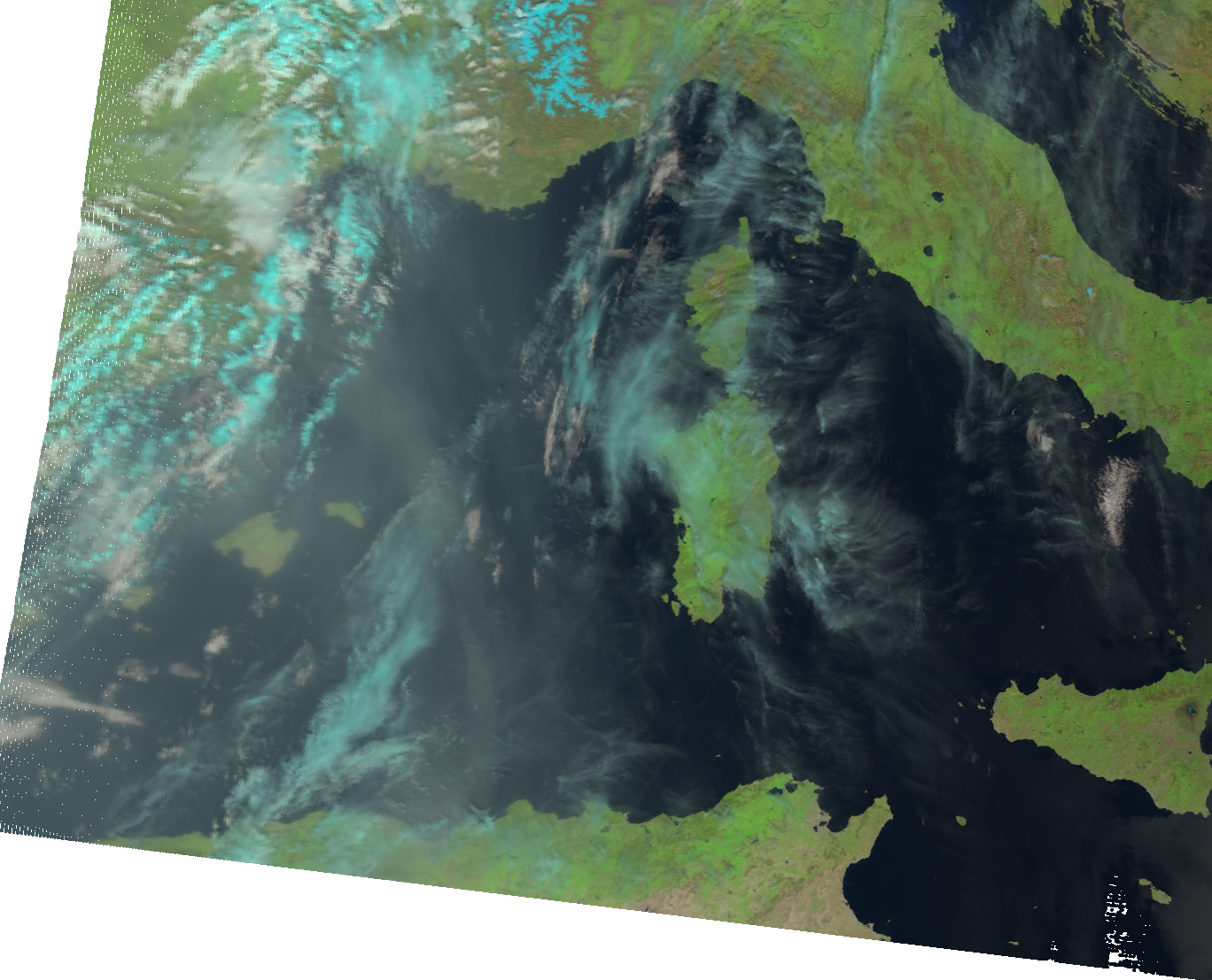
Afterwards, you can visualize the resampled natural_color RGB with the function show(). You see see dust intrusions over the Mediterranean sea.

scn_resample_nc.show('natural_color')

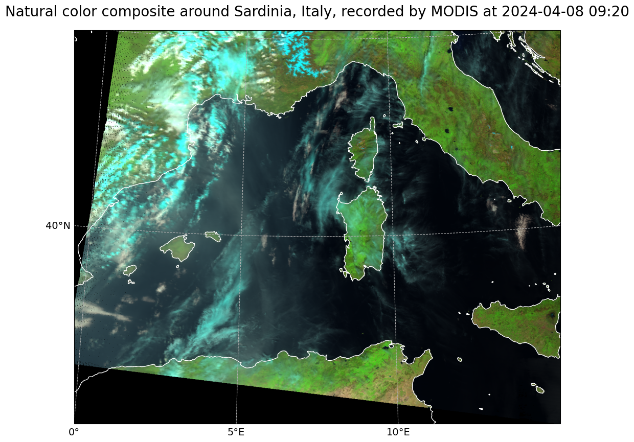
Visualize MODIS natural_color RGB composite with Cartopy features

SatPy’s built-in visualization function is nice, but often you want to make use of additonal features, such as country borders. The library Cartopy offers powerful functions that enable the visualization of geospatial data in different projections and to add additional features to a plot. Below, we will show you how you can visualize the natural_color composite with the two Python packages matplotlib and Cartopy.

As a first step, we have to convert the Scene object into a numpy array. The numpy array additionally needs to be transposed to a shape that can be interpreted by matplotlib’s function imshow(): (M,N,3). You can convert a Scene object into a numpy.array object with the function np.asarray().

The shape of the array is (3, 601, 667). This means we have to transpose the array and add index=0 on index position 3.

image = np.asarray(scn_resample_nc["natural_color"]).transpose(1,2,0)

The next step is then to replace all nan values with 0. You can do this with the numpy function nan_to_num(). In a subsequent step, we then scale the values to the range between 0 and 1, clipping the lower and upper percentiles so that a potential contrast decrease caused by outliers is eliminated.

image = np.nan_to_num(image)
image = np.interp(image, (np.percentile(image,1), np.percentile(image,99)), (0, 1))

Let us now also define a variable for the coordinate reference system. We take the area attribute from she scn_resample_nc Scene and convert it with the function to_cartopy_crs() into a format Cartopy can read. We will use the crs information for plotting.

crs = scn_resample_nc["natural_color"].attrs["area"].to_cartopy_crs()

Now, we can visualize the natural_color composite. The plotting code can be divided in four main parts:

• Initiate a matplotlib figure: Initiate a matplotlib plot and define the size of the plot

• Specify coastlines and a grid: specify additional features to be added to the plot

• Plotting function: plot the numpy array with the plotting function imshow()

• Set plot title: specify title of the plot

# ... and use it to generate an axes in our figure with the same CRS
fig = plt.figure(figsize=(16, 10))
ax = fig.add_subplot(1, 1, 1, projection=crs)

# Now we can add some coastlines...
ax.coastlines(resolution="10m", color="white")

# ... and a lat/lon grid:
gl = ax.gridlines(draw_labels=True, linestyle='--', xlocs=range(-10,11,5), ylocs=range(30,50,5))
gl.top_labels=False
gl.right_labels=False
gl.xformatter=LONGITUDE_FORMATTER
gl.yformatter=LATITUDE_FORMATTER
gl.xlabel_style={'size':14}
gl.ylabel_style={'size':14}

# In the end, we can plot our image data...
ax.imshow(image, transform=crs, extent=crs.bounds, origin="upper")

# and add a title to our plot
plt.title("Natural color composite around Sardinia, Italy, recorded by MODIS at " + scn_resample_nc.attrs["start_time"].strftime("%Y-%m-%d %H:%M"), fontsize=20, pad=20.0)

Text(0.5, 1.0, 'Natural color composite around Sardinia, Italy, recorded by MODIS at 2021-02-06 10:15')

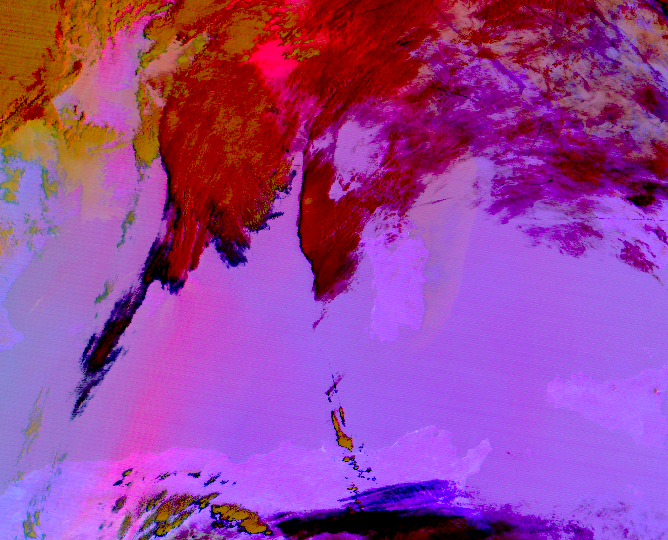
Visualize and interpret the ‘dust’ RGB composite

In a final step, we would like to have a closer look at the Dust RGB composite, whose primary aim is to support the detection of dust in the atmosphere. The dust composite makes use of three window channels:

• Red: IR12.0-IR10.8

• Green: IR10.8-IR.8.7

• Blue: IR10.8

Since we already loaded the dust composite to our Scene object scn_resample_nc, we can visualize the dust composite with Satpy’s built-in visualization function show(). The colours of the dust RGB can be interpreted as follows:

• Magenta: Dust or ash clouds

• Black: Cirrus clouds

• Dark red: Thick, high and cold ice clouds

• Yellow: Thick mid-level clouds

• Darkblue: Humid air in lower levels

• Lilac: Dry air in lower levels

Get more information about the Dust RGB in the SEVIRI Dust RGB Quick Guide.

The dust composite of 6 February at 10 UTC clearly show a dust cloud below the thicker cold ice cloud over northern Italy.

scn_resample_nc.show('dust')

previous

MSG SEVIRI RGB composites

next

Sentinel-5P TROPOMI UVAI