.ipynb .pdf

Contents

Solution 4

Hint

Execute the notebook on the training platform >>

About

So far, we analysed Aerosol Optical Depth from different types of data (satellite, model-based and ground-based observations) for a single dust event. Let us now broaden our view and analyse the annual cycle in 2020 of Aerosol Optical Depth from AERONET and compare it with the CAMS global reanalysis data.

Tasks

1. Download and plot time-series of AERONET data for Santa Cruz, Tenerife in 2020

• Hint

  • AERONET - Example notebook

  • you can select daily aggregates of the station observations by setting the AVG key to AVG=20

• Interpret the results:

  • Have there been other times in 2020 with increased AOD values?

  • If yes, how could you find out if the increase in AOD is caused by dust? Try to find out by visualizing the AOD time-series together with another parameter from the AERONET data.

  • MSG SEVIRI Dust RGB and MODIS RGB quick looks might be helpful to get a more complete picture of other events that might have happened in 2020

2. Download CAMS global reanalysis (EAC4) and select 2020 time-series for Santa Cruz, Tenerife

• Hint

  • CAMS global forecast - Example notebook (Note: the notebook works with CAMS forecast data, but they have a similar data structure to the CAMS global reanalysis data)

  • Data access with the following specifications:

  Variable on single levels: Dust aerosol optical depth at 550 nm
  Date: Start=2020-01-01, End=2020-12-31
  Time: [00:00, 03:00, 06:00, 09:00, 12:00, 15:00, 18:00, 21:00]
  Restricted area: N: 30., W: -20, E: 14, S: 20.
  Format: netCDF
  

  • With the xarray function sel() and keyword argument method='nearest' you can select data based on coordinate information

  • We also recommend you to transform your xarray.DataArray into a pandas.DataFrame with the function to_dataframe()

3. Visualize both time-series of CAMS reanalysis and AERONET daily aggregates in one plot

• Interpret the results: What can you say about the annual cycle in 2020 of AOD in Santa Cruz, Tenerife?

---

Load required libraries

import xarray as xr
import pandas as pd
import wget

from IPython.display import HTML

import matplotlib.pyplot as plt
import matplotlib.colors
from matplotlib.cm import get_cmap
from matplotlib import animation
from matplotlib.axes import Axes

import cartopy.crs as ccrs
from cartopy.mpl.gridliner import LONGITUDE_FORMATTER, LATITUDE_FORMATTER
import cartopy.feature as cfeature

from cartopy.mpl.geoaxes import GeoAxes
GeoAxes._pcolormesh_patched = Axes.pcolormesh

import warnings
warnings.simplefilter(action = "ignore", category = RuntimeWarning)

Load helper functions

%run ../../functions.ipynb

---

1. Download and plot time-series of AERONET data for Santa Cruz, Tenerife in 2020

Define latitude / longtiude values for Santa Cruz, Tenerife. You can see an overview of all available AERONET Site Names here.

lat = 28.473
lon = -16.247

As a first step, let us create a Python dictionary in which we store all the parameters we would like to use for the request as dictionary keys. You can initiate a dictionary with curled brackets {}. Below, we specify the following parameters:

• endpoint: Endpoint of the AERONET web service

• station: Name of the AERONET station

• year: year 1 of interest

• month: month 1 of interest

• day: day 1 of interest

• year2: year 2 of interest

• month2: month 2 of interest

• day2: day 2 of interest

• AOD15: data type, other options include AOD10, AOD20, etc.

• AVG: data format, AVG=10 - all points, AVG=20 - daily averages

The keywords below are those we will need for requesting daily averaged observations of Aerosol Optical Depth Level 1.5 data for the station Santa Cruz, Tenerife from 1 January to 31 December 2020.

data_dict = {
    'endpoint': 'https://aeronet.gsfc.nasa.gov/cgi-bin/print_web_data_v3',
    'station':'Santa_Cruz_Tenerife',
    'year': 2020,
    'month': 1,
    'day': 1,
    'year2': 2020,
    'month2': 12,
    'day2': 31,
    'AOD15': 1,
    'AVG': 20
}

In a next step, we construct the final string for the wget request with the format function. You construct a string by adding the dictionary keys in curled brackets. At the end of the string, you provide the dictionary key informatoin to the string with the format() function. A print of the resulting url shows, that the format function replaced the information in the curled brackets with the data in the dictionary.

url = '{endpoint}?site={station}&year={year}&month={month}&day={day}&year2={year2}&month2={month2}&day2={day2}&AOD15={AOD15}&AVG={AVG}'.format(**data_dict)
url

'https://aeronet.gsfc.nasa.gov/cgi-bin/print_web_data_v3?site=Santa_Cruz_Tenerife&year=2020&month=1&day=1&year2=2020&month2=12&day2=31&AOD15=1&AVG=20'

Now we are ready to request the data with the function download() from the wget Python library. You have to pass to the function the constructed url above together with a file path of where the downloaded that shall be stored. Let us store the data as txt file in the folder ../data/2_observations/aeronet/.

wget.download(url, '../../eodata/case_study/aeronet/2020_santa_cruz_tenerife_20.txt')

After we downloaded the station observations as txt file, we can open it with the pandas function read_table(). We additonally set specific keyword arguments that allow us to specify the columns and rows of interest:

• delimiter: specify the delimiter in the text file, e.g. comma

• header: specify the index of the row that shall be set as header.

• index_col: specify the index of the column that shall be set as index

You see below that the resulting dataframe has 296 rows and 81 columns.

df = pd.read_table('../../eodata/case_study/aeronet/2020_santa_cruz_tenerife_20.txt', delimiter=',', header=[7], index_col=1)
df

	AERONET_Site	Time(hh:mm:ss)	Day_of_Year	AOD_1640nm	AOD_1020nm	AOD_870nm	AOD_865nm	AOD_779nm	AOD_675nm	AOD_667nm	...	N[440-675_Angstrom_Exponent]	N[500-870_Angstrom_Exponent]	N[340-440_Angstrom_Exponent]	N[440-675_Angstrom_Exponent[Polar]]	Data_Quality_Level	AERONET_Instrument_Number	AERONET_Site_Name	Site_Latitude(Degrees)	Site_Longitude(Degrees)	Site_Elevation(m)<br>
Date(dd:mm:yyyy)
01:01:2020	Santa_Cruz_Tenerife	12:00:00	1.0	0.061198	0.076232	0.080599	-999.0	-999.0	0.085592	-999.0	...	87.0	87.0	87.0	0.0	lev15	1090.0	Santa_Cruz_Tenerife	28.472528	-16.247361	52.000000<br>
03:01:2020	Santa_Cruz_Tenerife	12:00:00	3.0	0.039688	0.052219	0.056409	-999.0	-999.0	0.063661	-999.0	...	131.0	131.0	131.0	0.0	lev15	1090.0	Santa_Cruz_Tenerife	28.472528	-16.247361	52.000000<br>
04:01:2020	Santa_Cruz_Tenerife	12:00:00	4.0	0.046246	0.058887	0.063752	-999.0	-999.0	0.073848	-999.0	...	39.0	39.0	39.0	0.0	lev15	1090.0	Santa_Cruz_Tenerife	28.472528	-16.247361	52.000000<br>
05:01:2020	Santa_Cruz_Tenerife	12:00:00	5.0	0.039780	0.050607	0.055417	-999.0	-999.0	0.065148	-999.0	...	59.0	59.0	58.0	0.0	lev15	1090.0	Santa_Cruz_Tenerife	28.472528	-16.247361	52.000000<br>
06:01:2020	Santa_Cruz_Tenerife	12:00:00	6.0	0.025086	0.033686	0.037128	-999.0	-999.0	0.042951	-999.0	...	33.0	33.0	32.0	0.0	lev15	1090.0	Santa_Cruz_Tenerife	28.472528	-16.247361	52.000000<br>
...	...	...	...	...	...	...	...	...	...	...	...	...	...	...	...	...	...	...	...	...	...
28:12:2020	Santa_Cruz_Tenerife	12:00:00	363.0	0.281631	0.361706	0.378314	-999.0	-999.0	0.398796	-999.0	...	95.0	95.0	95.0	0.0	lev15	1090.0	Santa_Cruz_Tenerife	28.472528	-16.247361	52.000000<br>
29:12:2020	Santa_Cruz_Tenerife	12:00:00	364.0	0.225135	0.279970	0.290588	-999.0	-999.0	0.304814	-999.0	...	35.0	35.0	35.0	0.0	lev15	1090.0	Santa_Cruz_Tenerife	28.472528	-16.247361	52.000000<br>
30:12:2020	Santa_Cruz_Tenerife	12:00:00	365.0	0.055233	0.075359	0.079524	-999.0	-999.0	0.086272	-999.0	...	34.0	34.0	34.0	0.0	lev15	1090.0	Santa_Cruz_Tenerife	28.472528	-16.247361	52.000000<br>
31:12:2020	Santa_Cruz_Tenerife	12:00:00	366.0	0.020104	0.025035	0.026090	-999.0	-999.0	0.028000	-999.0	...	56.0	56.0	55.0	0.0	lev15	1090.0	Santa_Cruz_Tenerife	28.472528	-16.247361	52.000000<br>
NaN	</body></html>	NaN	NaN	NaN	NaN	NaN	NaN	NaN	NaN	NaN	...	NaN	NaN	NaN	NaN	NaN	NaN	NaN	NaN	NaN	NaN

296 rows × 81 columns

Now, we can inspect the entries in the loaded data frame a bit more. Above you see that the last entry is a NaN entry, which is best to drop with the function dropna().

The next step is then to replace the entries with -999.0 and set them as NaN. We can use the function replace() to do so.

df = df.dropna()
df = df.replace(-999.0, np.nan)
df

	AERONET_Site	Time(hh:mm:ss)	Day_of_Year	AOD_1640nm	AOD_1020nm	AOD_870nm	AOD_865nm	AOD_779nm	AOD_675nm	AOD_667nm	...	N[440-675_Angstrom_Exponent]	N[500-870_Angstrom_Exponent]	N[340-440_Angstrom_Exponent]	N[440-675_Angstrom_Exponent[Polar]]	Data_Quality_Level	AERONET_Instrument_Number	AERONET_Site_Name	Site_Latitude(Degrees)	Site_Longitude(Degrees)	Site_Elevation(m)<br>
Date(dd:mm:yyyy)
01:01:2020	Santa_Cruz_Tenerife	12:00:00	1.0	0.061198	0.076232	0.080599	NaN	NaN	0.085592	NaN	...	87.0	87.0	87.0	0.0	lev15	1090.0	Santa_Cruz_Tenerife	28.472528	-16.247361	52.000000<br>
03:01:2020	Santa_Cruz_Tenerife	12:00:00	3.0	0.039688	0.052219	0.056409	NaN	NaN	0.063661	NaN	...	131.0	131.0	131.0	0.0	lev15	1090.0	Santa_Cruz_Tenerife	28.472528	-16.247361	52.000000<br>
04:01:2020	Santa_Cruz_Tenerife	12:00:00	4.0	0.046246	0.058887	0.063752	NaN	NaN	0.073848	NaN	...	39.0	39.0	39.0	0.0	lev15	1090.0	Santa_Cruz_Tenerife	28.472528	-16.247361	52.000000<br>
05:01:2020	Santa_Cruz_Tenerife	12:00:00	5.0	0.039780	0.050607	0.055417	NaN	NaN	0.065148	NaN	...	59.0	59.0	58.0	0.0	lev15	1090.0	Santa_Cruz_Tenerife	28.472528	-16.247361	52.000000<br>
06:01:2020	Santa_Cruz_Tenerife	12:00:00	6.0	0.025086	0.033686	0.037128	NaN	NaN	0.042951	NaN	...	33.0	33.0	32.0	0.0	lev15	1090.0	Santa_Cruz_Tenerife	28.472528	-16.247361	52.000000<br>
...	...	...	...	...	...	...	...	...	...	...	...	...	...	...	...	...	...	...	...	...	...
27:12:2020	Santa_Cruz_Tenerife	12:00:00	362.0	0.087975	0.114314	0.119534	NaN	NaN	0.125963	NaN	...	80.0	80.0	80.0	0.0	lev15	1090.0	Santa_Cruz_Tenerife	28.472528	-16.247361	52.000000<br>
28:12:2020	Santa_Cruz_Tenerife	12:00:00	363.0	0.281631	0.361706	0.378314	NaN	NaN	0.398796	NaN	...	95.0	95.0	95.0	0.0	lev15	1090.0	Santa_Cruz_Tenerife	28.472528	-16.247361	52.000000<br>
29:12:2020	Santa_Cruz_Tenerife	12:00:00	364.0	0.225135	0.279970	0.290588	NaN	NaN	0.304814	NaN	...	35.0	35.0	35.0	0.0	lev15	1090.0	Santa_Cruz_Tenerife	28.472528	-16.247361	52.000000<br>
30:12:2020	Santa_Cruz_Tenerife	12:00:00	365.0	0.055233	0.075359	0.079524	NaN	NaN	0.086272	NaN	...	34.0	34.0	34.0	0.0	lev15	1090.0	Santa_Cruz_Tenerife	28.472528	-16.247361	52.000000<br>
31:12:2020	Santa_Cruz_Tenerife	12:00:00	366.0	0.020104	0.025035	0.026090	NaN	NaN	0.028000	NaN	...	56.0	56.0	55.0	0.0	lev15	1090.0	Santa_Cruz_Tenerife	28.472528	-16.247361	52.000000<br>

295 rows × 81 columns

Let us now convert the index entry to a DateTimeIndex format with the function to_datetime(). Important here, you have to specify the format of the index string: %d:%m:%Y.

You see below that we do not have observations for every day. E.g on 2 January 2020, the data frame does not list any entry.

df.index = pd.to_datetime(df.index, format = '%d:%m:%Y')
df

	AERONET_Site	Time(hh:mm:ss)	Day_of_Year	AOD_1640nm	AOD_1020nm	AOD_870nm	AOD_865nm	AOD_779nm	AOD_675nm	AOD_667nm	...	N[440-675_Angstrom_Exponent]	N[500-870_Angstrom_Exponent]	N[340-440_Angstrom_Exponent]	N[440-675_Angstrom_Exponent[Polar]]	Data_Quality_Level	AERONET_Instrument_Number	AERONET_Site_Name	Site_Latitude(Degrees)	Site_Longitude(Degrees)	Site_Elevation(m)<br>
Date(dd:mm:yyyy)
2020-01-01	Santa_Cruz_Tenerife	12:00:00	1.0	0.061198	0.076232	0.080599	NaN	NaN	0.085592	NaN	...	87.0	87.0	87.0	0.0	lev15	1090.0	Santa_Cruz_Tenerife	28.472528	-16.247361	52.000000<br>
2020-01-03	Santa_Cruz_Tenerife	12:00:00	3.0	0.039688	0.052219	0.056409	NaN	NaN	0.063661	NaN	...	131.0	131.0	131.0	0.0	lev15	1090.0	Santa_Cruz_Tenerife	28.472528	-16.247361	52.000000<br>
2020-01-04	Santa_Cruz_Tenerife	12:00:00	4.0	0.046246	0.058887	0.063752	NaN	NaN	0.073848	NaN	...	39.0	39.0	39.0	0.0	lev15	1090.0	Santa_Cruz_Tenerife	28.472528	-16.247361	52.000000<br>
2020-01-05	Santa_Cruz_Tenerife	12:00:00	5.0	0.039780	0.050607	0.055417	NaN	NaN	0.065148	NaN	...	59.0	59.0	58.0	0.0	lev15	1090.0	Santa_Cruz_Tenerife	28.472528	-16.247361	52.000000<br>
2020-01-06	Santa_Cruz_Tenerife	12:00:00	6.0	0.025086	0.033686	0.037128	NaN	NaN	0.042951	NaN	...	33.0	33.0	32.0	0.0	lev15	1090.0	Santa_Cruz_Tenerife	28.472528	-16.247361	52.000000<br>
...	...	...	...	...	...	...	...	...	...	...	...	...	...	...	...	...	...	...	...	...	...
2020-12-27	Santa_Cruz_Tenerife	12:00:00	362.0	0.087975	0.114314	0.119534	NaN	NaN	0.125963	NaN	...	80.0	80.0	80.0	0.0	lev15	1090.0	Santa_Cruz_Tenerife	28.472528	-16.247361	52.000000<br>
2020-12-28	Santa_Cruz_Tenerife	12:00:00	363.0	0.281631	0.361706	0.378314	NaN	NaN	0.398796	NaN	...	95.0	95.0	95.0	0.0	lev15	1090.0	Santa_Cruz_Tenerife	28.472528	-16.247361	52.000000<br>
2020-12-29	Santa_Cruz_Tenerife	12:00:00	364.0	0.225135	0.279970	0.290588	NaN	NaN	0.304814	NaN	...	35.0	35.0	35.0	0.0	lev15	1090.0	Santa_Cruz_Tenerife	28.472528	-16.247361	52.000000<br>
2020-12-30	Santa_Cruz_Tenerife	12:00:00	365.0	0.055233	0.075359	0.079524	NaN	NaN	0.086272	NaN	...	34.0	34.0	34.0	0.0	lev15	1090.0	Santa_Cruz_Tenerife	28.472528	-16.247361	52.000000<br>
2020-12-31	Santa_Cruz_Tenerife	12:00:00	366.0	0.020104	0.025035	0.026090	NaN	NaN	0.028000	NaN	...	56.0	56.0	55.0	0.0	lev15	1090.0	Santa_Cruz_Tenerife	28.472528	-16.247361	52.000000<br>

295 rows × 81 columns

We can now plot the column AOD_500nm as annual time-series. You see that the station Santa Cruz, Tenerife was affected by other dust events later in 2020.

# Initiate a figure
fig = plt.figure(figsize=(20,8))
ax = plt.subplot()

# Define the plotting function
ax.plot(df.AOD_500nm, 'o-', color='green', label='AERONET observations')

# Customize the title and axes lables
ax.set_title('\nAerosol Optical Depth at 500 nm - Santa Cruz Tenerife\n', fontsize=20)
ax.set_ylabel('~', fontsize=14)
ax.set_xlabel('\nDay', fontsize=14)

# Customize the fontsize of the axes tickes
plt.xticks(fontsize=14)
plt.yticks(fontsize=14)

# Add a gridline to the plot
ax.grid(linestyle='--')

plt.legend(fontsize=16, loc=2)

<matplotlib.legend.Legend at 0x7f6faa4667c0>

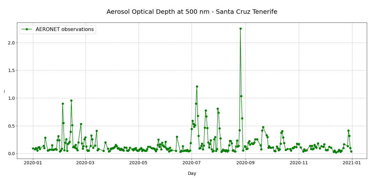
The next question is now, how you can find out, if the strong increase of AOD at the end of August 2020 was because of dust? For this to find out, you can use the Angstrom Exponent, which gives us an indication of the particle size. If the Angstrom Exponent is below 0.6, then it is an indication that the increase of AOD is caused by coarser dust particles.

Let us visualize the AOD at 500nm for 2020 together with the Angstrom Exponent 440-675nm.

# Initiate a figure
fig = plt.figure(figsize=(20,8))
ax = plt.subplot()

# Define the plotting function
ax.plot(df.AOD_500nm, 'o-', color='green', label='AERONET observations')
ax.plot(df['440-675_Angstrom_Exponent'], '-', color='lightgrey', label='Angstrom Exponent - 440-675nm')

plt.axhline(y=0.6, color='r', linestyle='dotted', label='Angstrom Exponent <0.6 is dust')

# Customize the title and axes lables
ax.set_title('\nAerosol Optical Depth at 500 nm - Santa Cruz Tenerife\n', fontsize=20)
ax.set_ylabel('~', fontsize=14)
ax.set_xlabel('\nDay', fontsize=14)

# Customize the fontsize of the axes tickes
plt.xticks(fontsize=14)
plt.yticks(fontsize=14)

# Add a gridline to the plot
ax.grid(linestyle='--')

plt.legend(fontsize=16, loc=2)

<matplotlib.legend.Legend at 0x7f23a7572700>

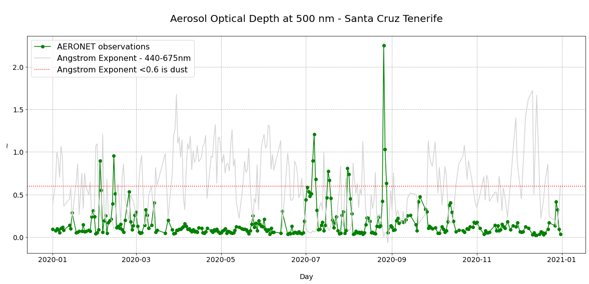
Above, you see that the Angstrom Exponent during the high AOD values at the end of August is very low. Hence, we could interpret this event as a strong dust intrusion. But is this really the case? You can also check here the MSG SEVIRI Dust RGB for e.g. 26 August 2020 and here the MODIS RGB to better understand the event and what could have caused the high AOD values.

2. Download CAMS global reanalysis (EAC4) and select 2020 time-series for Santa Cruz, Tenerife

First, we have to download the CAMS global reanalysis (EAC4) from the Copernicus Atmosphere Data Store with the following specifications:

• Variable on single levels: Dust aerosol optical depth at 550 nm

• Date: Start=2020-01-01, End=2020-12-31

• Time: [00:00, 03:00, 06:00, 09:00, 12:00, 15:00, 18:00, 21:00]

• Restricted area: N: 30., W: -20, E: 14, S: 20.

• Format: netCDF

See CDSAPI request below.

URL = 'https://ads.atmosphere.copernicus.eu/api/v2'
KEY = '######################'

import cdsapi

c = cdsapi.Client(url=URL, key=KEY)

c.retrieve(
    'cams-global-reanalysis-eac4',
    {
        'variable': 'dust_aerosol_optical_depth_550nm',
        'date': '2020-01-01/2020-12-31',
        'time': [
            '00:00', '03:00', '06:00',
            '09:00', '12:00', '15:00',
            '18:00', '21:00',
        ],
        'area': [
            30, -20, 20,
            15,
        ],
        'format': 'netcdf',
    },
    '../../eodata/case_study/cams/2020_dustAOD_cams_eac4.nc'}

The data is in netCDF, so we can open the netCDF file with the xarray function open_dataset(). We see that the data has three dimensions (latitude, longitude, time) and one data variable:

• duaod550: Dust Aerosol Optical Depth at 550nm

file = xr.open_dataset('../../eodata/case_study/cams/2020_dustAOD_cams_eac4.nc')
file

<xarray.Dataset>
Dimensions:    (latitude: 14, longitude: 47, time: 2928)
Coordinates:
  * longitude  (longitude) float32 -20.0 -19.25 -18.5 -17.75 ... 13.0 13.75 14.5
  * latitude   (latitude) float32 29.75 29.0 28.25 27.5 ... 21.5 20.75 20.0
  * time       (time) datetime64[ns] 2020-01-01 ... 2020-12-31T21:00:00
Data variables:
    duaod550   (time, latitude, longitude) float32 ...
Attributes:
    Conventions:  CF-1.6
    history:      2021-11-10 14:13:05 GMT by grib_to_netcdf-2.23.0: /opt/ecmw...

Let us now store the data variable Dust Aerosol Optical Depth (AOD) at 550nm as xarray.DataArray with the name duaod_cams.

duaod_cams = file['duaod550']
duaod_cams

<xarray.DataArray 'duaod550' (time: 2928, latitude: 14, longitude: 47)>
[1926624 values with dtype=float32]
Coordinates:
  * longitude  (longitude) float32 -20.0 -19.25 -18.5 -17.75 ... 13.0 13.75 14.5
  * latitude   (latitude) float32 29.75 29.0 28.25 27.5 ... 21.5 20.75 20.0
  * time       (time) datetime64[ns] 2020-01-01 ... 2020-12-31T21:00:00
Attributes:
    units:      ~
    long_name:  Dust Aerosol Optical Depth at 550nm

Now, we can select the time-series of the grid point nearest to the station in Santa Cruz, Tenerife. We can use the function sel() to select data based on the longitude and latitude dimensions. The keyword argument method='nearest' selects the grid point entry closest to the station coordinates.

cams_ts = duaod_cams.sel(longitude=lon, latitude=lat, method='nearest')
cams_ts

<xarray.DataArray 'duaod550' (time: 2928)>
array([0.007244, 0.021985, 0.060917, ..., 0.005728, 0.004677, 0.003822],
      dtype=float32)
Coordinates:
    longitude  float32 -16.25
    latitude   float32 28.25
  * time       (time) datetime64[ns] 2020-01-01 ... 2020-12-31T21:00:00
Attributes:
    units:      ~
    long_name:  Dust Aerosol Optical Depth at 550nm

The next step is now to resample the 3-hourly time entries and aggregate it to daily averages. We can use a combination of the functions resample() and mean() to create daily averages.

cams_ts_resample = cams_ts.resample(time='1D').mean()
cams_ts_resample

<xarray.DataArray 'duaod550' (time: 366)>
array([6.26771897e-02, 1.21897265e-01, 6.45051599e-02, 6.81166351e-03,
       1.11380219e-03, 2.36323476e-03, 1.70692801e-03, 2.12018192e-03,
       2.59661674e-03, 1.27915293e-02, 2.31949985e-03, 1.18672848e-03,
       6.82000369e-02, 9.66019481e-02, 1.06641322e-01, 5.51756322e-02,
       6.65611029e-03, 3.57866287e-03, 5.35264611e-04, 5.40107489e-04,
       1.26868486e-04, 2.28971243e-04, 5.88308275e-03, 7.26868212e-03,
       6.05811179e-03, 4.26903367e-03, 1.19990855e-02, 9.62656736e-03,
       8.38011652e-02, 1.65890560e-01, 1.58602878e-01, 6.69117123e-02,
       4.65308130e-03, 7.19046295e-02, 3.36282521e-01, 3.49263191e-01,
       8.95184875e-02, 6.27355129e-02, 1.27191618e-01, 1.28401518e-02,
       2.42699534e-02, 7.66301751e-02, 1.55321255e-01, 2.17939615e-01,
       4.48830277e-01, 3.32869619e-01, 6.46899045e-02, 5.61430752e-02,
       2.86746323e-02, 1.25387311e-02, 2.85427272e-03, 4.57480550e-04,
       1.68058857e-01, 7.46165454e-01, 5.34614563e-01, 4.31294233e-01,
       1.71836376e-01, 5.27052581e-03, 2.51790732e-02, 1.20623484e-01,
       1.22927919e-01, 5.87635338e-02, 9.09666717e-03, 1.24505162e-03,
       9.78703797e-03, 1.80081427e-02, 3.58837843e-03, 1.31649762e-01,
       1.49847046e-01, 5.58611155e-02, 8.08890164e-02, 1.23239055e-01,
       1.12538531e-01, 1.09684721e-01, 2.63993740e-02, 5.64485788e-03,
       1.56059861e-04, 5.24136424e-03, 1.17954418e-01, 1.49613649e-01,
...
       1.51704177e-01, 9.84493941e-02, 4.13101166e-02, 2.73425579e-02,
       4.11496758e-02, 9.22799408e-02, 2.60631740e-03, 1.46314502e-04,
       1.17123127e-04, 8.80983472e-03, 8.88815969e-02, 9.45503116e-02,
       3.46885324e-02, 3.57580930e-02, 4.34055179e-02, 9.80604440e-02,
       2.00432733e-01, 8.51429701e-02, 5.67653924e-02, 8.52298737e-03,
       4.79409099e-03, 3.50505114e-04, 1.65790319e-04, 5.30421734e-04,
       9.14469361e-04, 1.81388855e-03, 5.34346700e-03, 2.23447382e-02,
       2.38129646e-02, 5.62014282e-02, 1.12864256e-01, 6.75437450e-02,
       1.27838194e-01, 6.38682693e-02, 5.41449189e-02, 5.96240610e-02,
       5.70862293e-02, 7.16469884e-02, 3.21166962e-02, 5.39456010e-02,
       1.17779389e-01, 7.62315542e-02, 5.20691276e-04, 5.88297844e-05,
       1.17167830e-04, 3.99127603e-04, 8.31186771e-05, 3.01882625e-04,
       3.35916877e-04, 1.56059861e-04, 1.38117373e-03, 3.31127644e-03,
       3.93986702e-05, 7.88062811e-04, 3.60235572e-04, 2.97054648e-04,
       2.97039747e-04, 2.58132815e-04, 6.32479787e-04, 6.32479787e-04,
       3.45647335e-04, 1.31756067e-04, 4.42564487e-05, 1.07407570e-04,
       1.12280250e-04, 1.02549791e-04, 1.26838684e-04, 7.34031200e-05,
       1.72642767e-02, 1.09888896e-01, 2.62545496e-01, 3.42311025e-01,
       9.04908031e-02, 6.92404509e-02, 2.15455323e-01, 1.82337582e-01,
       7.28429556e-02, 1.04822367e-02], dtype=float32)
Coordinates:
  * time       (time) datetime64[ns] 2020-01-01 2020-01-02 ... 2020-12-31
    longitude  float32 -16.25
    latitude   float32 28.25

A closer look at the time dimension shows us that we now have an entry for each day in 2020.

cams_ts_resample.time

<xarray.DataArray 'time' (time: 366)>
array(['2020-01-01T00:00:00.000000000', '2020-01-02T00:00:00.000000000',
       '2020-01-03T00:00:00.000000000', ..., '2020-12-29T00:00:00.000000000',
       '2020-12-30T00:00:00.000000000', '2020-12-31T00:00:00.000000000'],
      dtype='datetime64[ns]')
Coordinates:
  * time       (time) datetime64[ns] 2020-01-01 2020-01-02 ... 2020-12-31
    longitude  float32 -16.25
    latitude   float32 28.25

Now, we can convert the xarray.DataArray to a pandas.DataFrame, as pandas is more efficient to handle time-series data. The function to_dataframe() easily converts a data array to a dataframe. The resulting dataframe has 366 rows and 3 columns.

cams_ts_df = cams_ts_resample.to_dataframe()
cams_ts_df

	longitude	latitude	duaod550
time
2020-01-01	-16.25	28.25	0.062677
2020-01-02	-16.25	28.25	0.121897
2020-01-03	-16.25	28.25	0.064505
2020-01-04	-16.25	28.25	0.006812
2020-01-05	-16.25	28.25	0.001114
...	...	...	...
2020-12-27	-16.25	28.25	0.069240
2020-12-28	-16.25	28.25	0.215455
2020-12-29	-16.25	28.25	0.182338
2020-12-30	-16.25	28.25	0.072843
2020-12-31	-16.25	28.25	0.010482

366 rows × 3 columns

3. Combine both annual time-series and visualize both in one plot

Let us now use the function join() and combine the two time-series cams_ts_df and df['AOD_500nm]. The resulting dataframe has 366 rows and 4 columns.

df_combined = cams_ts_df.join(df['AOD_500nm'])
df_combined

	longitude	latitude	duaod550	AOD_500nm
time
2020-01-01	-16.25	28.25	0.062677	0.094487
2020-01-02	-16.25	28.25	0.121897	NaN
2020-01-03	-16.25	28.25	0.064505	0.075765
2020-01-04	-16.25	28.25	0.006812	0.098110
2020-01-05	-16.25	28.25	0.001114	0.085672
...	...	...	...	...
2020-12-27	-16.25	28.25	0.069240	0.134366
2020-12-28	-16.25	28.25	0.215455	0.415433
2020-12-29	-16.25	28.25	0.182338	0.320463
2020-12-30	-16.25	28.25	0.072843	0.095342
2020-12-31	-16.25	28.25	0.010482	0.033297

366 rows × 4 columns

Let us safe the pandas dataframe as csv file. This allows us to easily load the time-series again at a later stage. You can use the function to_csv() to save a pandas.DataFrame as csv.

df_combined.to_csv("../../eodata/case_study/2020_ts_cams_aeronet.csv", index_label='time')

The last step is now to plot the two columns of the pandas.DataFrame df_combined as two individual line plots.

# Initiate a figure
fig = plt.figure(figsize=(20,8))
ax = plt.subplot()

# Define the plotting function
ax.plot(df_combined.duaod550, '-', color='blue', label='CAMS global reanalysis (EAC4) - 550 nm')
ax.plot(df_combined.AOD_500nm, '-', color='green', label='AERONET observations - 500 nm')
plt.axhline(y=0.6, color='r', linestyle='dotted', label='PM10 daily limit')

# Customize the title and axes lables
ax.set_title('\nAerosol Optical Depth at 500 / 550 nm - Santa Cruz Tenerife\n', fontsize=20)
ax.set_ylabel(cams_ts.units, fontsize=14)
ax.set_xlabel('\nDay', fontsize=14)

# Customize the fontsize of the axes tickes
plt.xticks(fontsize=14)
plt.yticks(fontsize=14)

# Add a gridline to the plot
ax.grid(linestyle='--')

plt.legend(fontsize=14, loc=2)

<matplotlib.legend.Legend at 0x7f13c625a070>

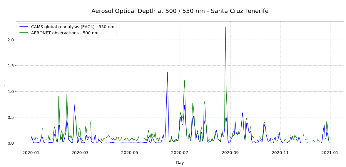
You see in the plot above that the model and the AERONET observations follow a similar annual cycle of AOD in 2020 for the Santa Cruz station in Tenerife. You also see that for higher AOD values measured by AERONET, the CAMS model mostly underpredicts the AOD intensity.

previous

Solution 3

next

Solution 5