Solution 2#
About#
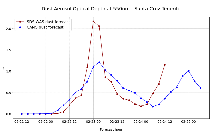
Let us have a closer look at the forecast data from both models for one observation station in Tenerife (Canary Islands). Let us plot the time-series of the CAMS and MONARCH forecasts together in one plot.
Tasks#
1. Download and animate the CAMS global forecast for 21 Feb 2020
Download the CAMS global atmospheric composition forecast for 21 February 2020, with the following specifications:
Variable on single levels:
Dust aerosol optical depth at 550 nm
Date (Start and end):2020-02-21
Time:12:00
Leadtime hour: every three hours from0 to 90
Type:Forecast
Restricted area:N: 67, W: -30, E: 71, S: -3
Format:Zipped netCDFHint
2. Get the coordinates of the AERONET station Santa Cruz, Tenerife
Hint
You can see an overview of all available AERONET Site Names here
3. Select the time-series for CAMS global atmospheric composition forecasts for Santa Cruz, Tenerife
Hint
With the xarray function
sel()and keyword argumentmethod='nearest'you can select data based on coordinate informationWe also recommend you to transform your xarray.DataArray into a pandas.DataFrame with the function
to_dataframe()and save it ascsvwith the functionto_csv()
4. Load the MONARCH dust forecasts and select time-series for Santa Cruz, Tenerife
Hint
With the xarray function
sel()and keyword argumentmethod='nearest'you can select data based on coordinate informationWe also recommend you to transform your xarray.DataArray into a pandas.DataFrame with the function
to_dataframe()and save it ascsvwith the functionto_csv()
5. Visualize both time-series of CAMS and MONARCH forecasts together in one plot
Load required libraries
import xarray as xr
import pandas as pd

from IPython.display import HTML

import matplotlib.pyplot as plt
import matplotlib.colors
from matplotlib.cm import get_cmap
from matplotlib import animation
from matplotlib.axes import Axes

import cartopy.crs as ccrs
from cartopy.mpl.gridliner import LONGITUDE_FORMATTER, LATITUDE_FORMATTER
import cartopy.feature as cfeature
from cartopy.mpl.geoaxes import GeoAxes
GeoAxes._pcolormesh_patched = Axes.pcolormesh

import warnings
warnings.simplefilter(action = "ignore", category = RuntimeWarning)
Load helper functions
%run ../../functions.ipynb
1. Download and animate the CAMS global forecast for 21 Feb 2020#
First, we have to download the CAMS global atmospheric composition forecast data from the Copernicus Atmosphere Data Store with the following specifications:
Variable on single levels:
Dust aerosol optical depth at 550 nmDate (Start and end):
2020-02-21Time:
12:00Leadtime hour: every three hours from
0 to 90Type:
ForecastRestricted area:
N: 67, W: -30, E: 71, S: -3Format:
Zipped netCDF
See the CDSAPI request below.
URL = 'https://ads.atmosphere.copernicus.eu/api/v2'
KEY = '######################'
import cdsapi

c = cdsapi.Client(url=URL, key=KEY)

c.retrieve(
    'cams-global-atmospheric-composition-forecasts',
    {
        'variable': 'dust_aerosol_optical_depth_550nm',
        'date': '2020-02-21/2020-02-21',
        'time': '12:00',
        'leadtime_hour': [
            '0', '12', '15',
            '18', '21', '24',
            '27', '3', '30',
            '33', '36', '39',
            '42', '45', '48',
            '51', '54', '57',
            '6', '60', '63',
            '66', '69', '72',
            '75', '78', '81',
            '84', '87', '9',
            '90',
        ],
        'type': 'forecast',
        'area': [
            67, -30, -3,
            71,
        ],
        'format': 'netcdf_zip',
    },
    '../../eodata/case_study/cams/20210221_dustAOD.zip')
The first step is to unzip file from the zipped archive downloaded.
import zipfile
with zipfile.ZipFile('../../eodata/case_study/cams/20200221_dustAOD.zip', 'r') as zip_ref:
    zip_ref.extractall('../../')
Then, we can open the netCDF file with the xarray function open_dataset(). We see that the data has three dimensions (latitude, longitude, time) and one data variable:
duaod550: Dust Aerosol Optical Depth at 550nm
file = xr.open_dataset('../../eodata/case_study/cams/data.nc')
file
<xarray.Dataset>
Dimensions:    (longitude: 253, latitude: 176, time: 31)
Coordinates:
  * longitude  (longitude) float32 -30.0 -29.6 -29.2 -28.8 ... 70.0 70.4 70.8
  * latitude   (latitude) float32 67.0 66.6 66.2 65.8 ... -1.8 -2.2 -2.6 -3.0
  * time       (time) datetime64[ns] 2020-02-21T12:00:00 ... 2020-02-25T06:00:00
Data variables:
    duaod550   (time, latitude, longitude) float32 ...
Attributes:
    Conventions:  CF-1.6
history: 2021-11-02 14:50:00 GMT by grib_to_netcdf-2.23.0: /opt/ecmw...- longitude: 253
- latitude: 176
- time: 31
- longitude(longitude)float32-30.0 -29.6 -29.2 ... 70.4 70.8
- units :
- degrees_east
- long_name :
- longitude
array([-30. , -29.6, -29.2, ..., 70. , 70.4, 70.8], dtype=float32)
- latitude(latitude)float3267.0 66.6 66.2 ... -2.2 -2.6 -3.0
- units :
- degrees_north
- long_name :
- latitude
array([67. , 66.6, 66.2, 65.8, 65.4, 65. , 64.6, 64.2, 63.8, 63.4, 63. , 62.6, 62.2, 61.8, 61.4, 61. , 60.6, 60.2, 59.8, 59.4, 59. , 58.6, 58.2, 57.8, 57.4, 57. , 56.6, 56.2, 55.8, 55.4, 55. , 54.6, 54.2, 53.8, 53.4, 53. , 52.6, 52.2, 51.8, 51.4, 51. , 50.6, 50.2, 49.8, 49.4, 49. , 48.6, 48.2, 47.8, 47.4, 47. , 46.6, 46.2, 45.8, 45.4, 45. , 44.6, 44.2, 43.8, 43.4, 43. , 42.6, 42.2, 41.8, 41.4, 41. , 40.6, 40.2, 39.8, 39.4, 39. , 38.6, 38.2, 37.8, 37.4, 37. , 36.6, 36.2, 35.8, 35.4, 35. , 34.6, 34.2, 33.8, 33.4, 33. , 32.6, 32.2, 31.8, 31.4, 31. , 30.6, 30.2, 29.8, 29.4, 29. , 28.6, 28.2, 27.8, 27.4, 27. , 26.6, 26.2, 25.8, 25.4, 25. , 24.6, 24.2, 23.8, 23.4, 23. , 22.6, 22.2, 21.8, 21.4, 21. , 20.6, 20.2, 19.8, 19.4, 19. , 18.6, 18.2, 17.8, 17.4, 17. , 16.6, 16.2, 15.8, 15.4, 15. , 14.6, 14.2, 13.8, 13.4, 13. , 12.6, 12.2, 11.8, 11.4, 11. , 10.6, 10.2, 9.8, 9.4, 9. , 8.6, 8.2, 7.8, 7.4, 7. , 6.6, 6.2, 5.8, 5.4, 5. , 4.6, 4.2, 3.8, 3.4, 3. , 2.6, 2.2, 1.8, 1.4, 1. , 0.6, 0.2, -0.2, -0.6, -1. , -1.4, -1.8, -2.2, -2.6, -3. ], dtype=float32) - time(time)datetime64[ns]2020-02-21T12:00:00 ... 2020-02-...
- long_name :
- time
array(['2020-02-21T12:00:00.000000000', '2020-02-21T15:00:00.000000000',
       '2020-02-21T18:00:00.000000000', '2020-02-21T21:00:00.000000000',
       '2020-02-22T00:00:00.000000000', '2020-02-22T03:00:00.000000000',
       '2020-02-22T06:00:00.000000000', '2020-02-22T09:00:00.000000000',
       '2020-02-22T12:00:00.000000000', '2020-02-22T15:00:00.000000000',
       '2020-02-22T18:00:00.000000000', '2020-02-22T21:00:00.000000000',
       '2020-02-23T00:00:00.000000000', '2020-02-23T03:00:00.000000000',
       '2020-02-23T06:00:00.000000000', '2020-02-23T09:00:00.000000000',
       '2020-02-23T12:00:00.000000000', '2020-02-23T15:00:00.000000000',
       '2020-02-23T18:00:00.000000000', '2020-02-23T21:00:00.000000000',
       '2020-02-24T00:00:00.000000000', '2020-02-24T03:00:00.000000000',
       '2020-02-24T06:00:00.000000000', '2020-02-24T09:00:00.000000000',
       '2020-02-24T12:00:00.000000000', '2020-02-24T15:00:00.000000000',
       '2020-02-24T18:00:00.000000000', '2020-02-24T21:00:00.000000000',
       '2020-02-25T00:00:00.000000000', '2020-02-25T03:00:00.000000000',
       '2020-02-25T06:00:00.000000000'], dtype='datetime64[ns]')
- duaod550(time, latitude, longitude)float32...
- units :
- ~
- long_name :
- Dust Aerosol Optical Depth at 550nm
[1380368 values with dtype=float32]
- Conventions :
- CF-1.6
- history :
- 2021-11-02 14:50:00 GMT by grib_to_netcdf-2.23.0: /opt/ecmwf/mars-client/bin/grib_to_netcdf -S param -o /cache/tmp/b8f9e27f-7176-4f09-b29d-111ed06138e8-adaptor.mars_constrained.external-1635864600.6827648-13866-24-tmp.nc /cache/tmp/b8f9e27f-7176-4f09-b29d-111ed06138e8-adaptor.mars_constrained.external-1635864600.6122434-13866-23-tmp.grib
Let us now store the data variable Dust Aerosol Optical Depth (AOD) at 550nm as xarray.DataArray with the name du_aod.
du_aod = file.duaod550
du_aod
<xarray.DataArray 'duaod550' (time: 31, latitude: 176, longitude: 253)>
[1380368 values with dtype=float32]
Coordinates:
  * longitude  (longitude) float32 -30.0 -29.6 -29.2 -28.8 ... 70.0 70.4 70.8
  * latitude   (latitude) float32 67.0 66.6 66.2 65.8 ... -1.8 -2.2 -2.6 -3.0
  * time       (time) datetime64[ns] 2020-02-21T12:00:00 ... 2020-02-25T06:00:00
Attributes:
    units:      ~
long_name: Dust Aerosol Optical Depth at 550nm- time: 31
- latitude: 176
- longitude: 253
- ...
[1380368 values with dtype=float32]
- longitude(longitude)float32-30.0 -29.6 -29.2 ... 70.4 70.8
- units :
- degrees_east
- long_name :
- longitude
array([-30. , -29.6, -29.2, ..., 70. , 70.4, 70.8], dtype=float32)
- latitude(latitude)float3267.0 66.6 66.2 ... -2.2 -2.6 -3.0
- units :
- degrees_north
- long_name :
- latitude
array([67. , 66.6, 66.2, 65.8, 65.4, 65. , 64.6, 64.2, 63.8, 63.4, 63. , 62.6, 62.2, 61.8, 61.4, 61. , 60.6, 60.2, 59.8, 59.4, 59. , 58.6, 58.2, 57.8, 57.4, 57. , 56.6, 56.2, 55.8, 55.4, 55. , 54.6, 54.2, 53.8, 53.4, 53. , 52.6, 52.2, 51.8, 51.4, 51. , 50.6, 50.2, 49.8, 49.4, 49. , 48.6, 48.2, 47.8, 47.4, 47. , 46.6, 46.2, 45.8, 45.4, 45. , 44.6, 44.2, 43.8, 43.4, 43. , 42.6, 42.2, 41.8, 41.4, 41. , 40.6, 40.2, 39.8, 39.4, 39. , 38.6, 38.2, 37.8, 37.4, 37. , 36.6, 36.2, 35.8, 35.4, 35. , 34.6, 34.2, 33.8, 33.4, 33. , 32.6, 32.2, 31.8, 31.4, 31. , 30.6, 30.2, 29.8, 29.4, 29. , 28.6, 28.2, 27.8, 27.4, 27. , 26.6, 26.2, 25.8, 25.4, 25. , 24.6, 24.2, 23.8, 23.4, 23. , 22.6, 22.2, 21.8, 21.4, 21. , 20.6, 20.2, 19.8, 19.4, 19. , 18.6, 18.2, 17.8, 17.4, 17. , 16.6, 16.2, 15.8, 15.4, 15. , 14.6, 14.2, 13.8, 13.4, 13. , 12.6, 12.2, 11.8, 11.4, 11. , 10.6, 10.2, 9.8, 9.4, 9. , 8.6, 8.2, 7.8, 7.4, 7. , 6.6, 6.2, 5.8, 5.4, 5. , 4.6, 4.2, 3.8, 3.4, 3. , 2.6, 2.2, 1.8, 1.4, 1. , 0.6, 0.2, -0.2, -0.6, -1. , -1.4, -1.8, -2.2, -2.6, -3. ], dtype=float32) - time(time)datetime64[ns]2020-02-21T12:00:00 ... 2020-02-...
- long_name :
- time
array(['2020-02-21T12:00:00.000000000', '2020-02-21T15:00:00.000000000',
       '2020-02-21T18:00:00.000000000', '2020-02-21T21:00:00.000000000',
       '2020-02-22T00:00:00.000000000', '2020-02-22T03:00:00.000000000',
       '2020-02-22T06:00:00.000000000', '2020-02-22T09:00:00.000000000',
       '2020-02-22T12:00:00.000000000', '2020-02-22T15:00:00.000000000',
       '2020-02-22T18:00:00.000000000', '2020-02-22T21:00:00.000000000',
       '2020-02-23T00:00:00.000000000', '2020-02-23T03:00:00.000000000',
       '2020-02-23T06:00:00.000000000', '2020-02-23T09:00:00.000000000',
       '2020-02-23T12:00:00.000000000', '2020-02-23T15:00:00.000000000',
       '2020-02-23T18:00:00.000000000', '2020-02-23T21:00:00.000000000',
       '2020-02-24T00:00:00.000000000', '2020-02-24T03:00:00.000000000',
       '2020-02-24T06:00:00.000000000', '2020-02-24T09:00:00.000000000',
       '2020-02-24T12:00:00.000000000', '2020-02-24T15:00:00.000000000',
       '2020-02-24T18:00:00.000000000', '2020-02-24T21:00:00.000000000',
       '2020-02-25T00:00:00.000000000', '2020-02-25T03:00:00.000000000',
       '2020-02-25T06:00:00.000000000'], dtype='datetime64[ns]')
- units :
- ~
- long_name :
- Dust Aerosol Optical Depth at 550nm
Above, you see that the variable du_aod has two attributes, units and long_name. Let us define variables for those attributes. The variables can be used for visualizing the data.
long_name = du_aod.long_name
units = du_aod.units
Let us do the same for the coordinates longitude and latitude.
latitude = du_aod.latitude
longitude = du_aod.longitude
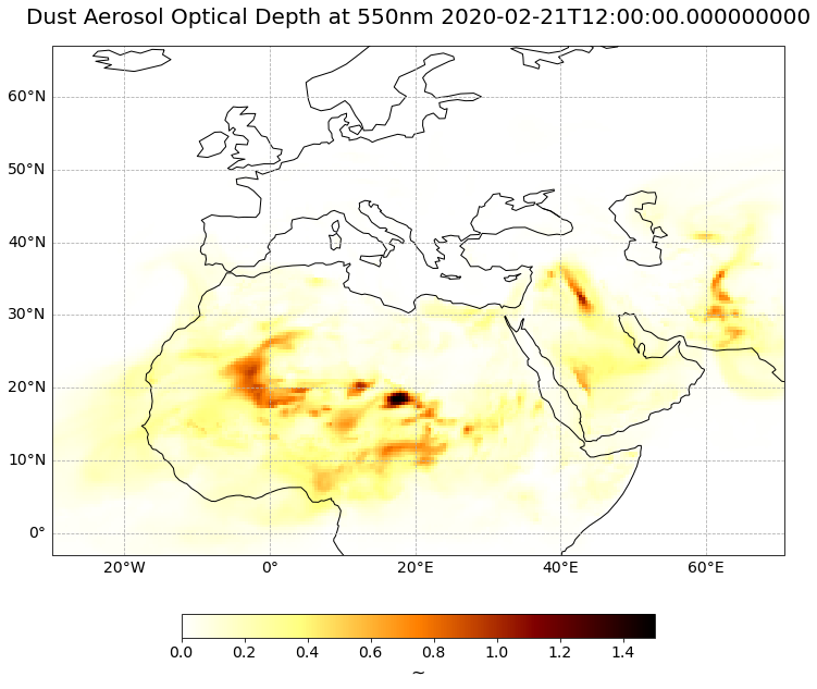
Visualize one forecast step of Dust Aerosol Optical Depth at 550nm
The next step is to visualize the dataset. You can use the function visualize_pcolormesh, which makes use of matploblib’s function pcolormesh and the Cartopy library.
visualize_pcolormesh(data_array=du_aod[0,:,:],
                     longitude=longitude,
                     latitude=latitude,
                     projection=ccrs.PlateCarree(),
                     color_scale='afmhot_r',
                     unit=units,
                     long_name=long_name + ' ' + str(du_aod[0,:,:].time.data),
                     vmin=0,
                     vmax=1.5,
                     set_global=False,
                    lonmin=du_aod.longitude.min(),
                    lonmax=du_aod.longitude.max(),
                    latmin=du_aod.latitude.min(),
                    latmax=du_aod.latitude.max())
(<Figure size 1440x720 with 2 Axes>,
 <GeoAxesSubplot:title={'center':'Dust Aerosol Optical Depth at 550nm 2020-02-21T12:00:00.000000000'}>)
Now, we can also animate the forecast. The animation function consists of 4 parts:
Setting the initial state:
Here, you define the general plot your animation shall use to initialise the animation. You can also define the number of frames (time steps) your animation shall have.Functions to animate:
An animation consists of three functions:draw(),init()andanimate().draw()is the function where individual frames are passed on and the figure is returned as image. In this example, the function redraws the plot for each time step.init()returns the figure you defined for the initial state.animate()returns thedraw()function and animates the function over the given number of frames (time steps).Create a
animate.FuncAnimationobject:
The functions defined before are now combined to build ananimate.FuncAnimationobject.Play the animation as video:
As a final step, you can integrate the animation into the notebook with theHTMLclass. You take the generate animation object and convert it to a HTML5 video with theto_html5_videofunction
# Setting the initial state:
# 1. Define figure for initial plot
fig, ax = visualize_pcolormesh(data_array=du_aod[0,:,:],
                               longitude=du_aod.longitude,
                               latitude=du_aod.latitude,
                               projection=ccrs.PlateCarree(),
                               color_scale='afmhot_r',
                               unit='-',
                               long_name=long_name + ' '+ str(du_aod.time[0].data),
                               vmin=0,
                               vmax=1,
                                lonmin=du_aod.longitude.min(),
                                lonmax=du_aod.longitude.max(),
                                latmin=du_aod.latitude.min(),
                                latmax=du_aod.latitude.max(),
                               set_global=False)

frames = 30

def draw(i):
    img = plt.pcolormesh(du_aod.longitude,
                         du_aod.latitude,
                         du_aod[i,:,:],
                         cmap='afmhot_r',
                         transform=ccrs.PlateCarree(),
                         vmin=0,
                         vmax=1,
                         shading='auto')

    ax.set_title(long_name + ' '+ str(du_aod.time[i].data), fontsize=20, pad=20.0)
    return img


def init():
    return fig


def animate(i):
    return draw(i)

ani = animation.FuncAnimation(fig, animate, frames, interval=800, blit=False,
                              init_func=init, repeat=True)

HTML(ani.to_html5_video())
plt.close(fig)
Play the animation video as HTML5 video
HTML(ani.to_html5_video())
2. Select latitude / longitude values for Santa Cruz, Tenerife#
You can see an overview of all available AERONET Site Names here. Let’s look up the latitude and longitude information for the station Santa_Cruz_Tenerife and define the coordinate information as variables.
lat = 28.473
lon = -16.247
3. Select the time-series for CAMS global atmospheric composition forecasts for Santa Cruz, Tenerife#
From the loaded xarray data array du_aod, we can now select the values for one specific point location. We can select coordinate information with the function sel(). We have to make sure to set the keyword argument method='nearest'. With this keyword argument, the closest grid location in the data array is used for the time-series retrieval.
cams_ts = du_aod.sel(longitude=lon, latitude=lat, method='nearest')
cams_ts
<xarray.DataArray 'duaod550' (time: 31)>
array([5.676746e-04, 5.676746e-04, 1.460314e-03, 2.421856e-03, 5.305767e-03,
       1.128006e-02, 8.077216e-02, 2.031391e-01, 3.358061e-01, 5.017774e-01,
       5.811578e-01, 7.555066e-01, 1.102213e+00, 1.210434e+00, 1.024824e+00,
       9.059588e-01, 7.769997e-01, 6.033378e-01, 5.451070e-01, 4.923698e-01,
       3.647155e-01, 2.810775e-01, 1.702471e-01, 2.191389e-01, 3.551019e-01,
       5.156484e-01, 6.221528e-01, 8.869376e-01, 1.008824e+00, 7.652575e-01,
       6.062905e-01], dtype=float32)
Coordinates:
    longitude  float32 -16.4
    latitude   float32 28.6
  * time       (time) datetime64[ns] 2020-02-21T12:00:00 ... 2020-02-25T06:00:00
Attributes:
    units:      ~
long_name: Dust Aerosol Optical Depth at 550nm- time: 31
- 0.0005677 0.0005677 0.00146 0.002422 ... 0.8869 1.009 0.7653 0.6063
array([5.676746e-04, 5.676746e-04, 1.460314e-03, 2.421856e-03, 5.305767e-03, 1.128006e-02, 8.077216e-02, 2.031391e-01, 3.358061e-01, 5.017774e-01, 5.811578e-01, 7.555066e-01, 1.102213e+00, 1.210434e+00, 1.024824e+00, 9.059588e-01, 7.769997e-01, 6.033378e-01, 5.451070e-01, 4.923698e-01, 3.647155e-01, 2.810775e-01, 1.702471e-01, 2.191389e-01, 3.551019e-01, 5.156484e-01, 6.221528e-01, 8.869376e-01, 1.008824e+00, 7.652575e-01, 6.062905e-01], dtype=float32) - longitude()float32-16.4
- units :
- degrees_east
- long_name :
- longitude
array(-16.4, dtype=float32)
- latitude()float3228.6
- units :
- degrees_north
- long_name :
- latitude
array(28.6, dtype=float32)
- time(time)datetime64[ns]2020-02-21T12:00:00 ... 2020-02-...
- long_name :
- time
array(['2020-02-21T12:00:00.000000000', '2020-02-21T15:00:00.000000000',
       '2020-02-21T18:00:00.000000000', '2020-02-21T21:00:00.000000000',
       '2020-02-22T00:00:00.000000000', '2020-02-22T03:00:00.000000000',
       '2020-02-22T06:00:00.000000000', '2020-02-22T09:00:00.000000000',
       '2020-02-22T12:00:00.000000000', '2020-02-22T15:00:00.000000000',
       '2020-02-22T18:00:00.000000000', '2020-02-22T21:00:00.000000000',
       '2020-02-23T00:00:00.000000000', '2020-02-23T03:00:00.000000000',
       '2020-02-23T06:00:00.000000000', '2020-02-23T09:00:00.000000000',
       '2020-02-23T12:00:00.000000000', '2020-02-23T15:00:00.000000000',
       '2020-02-23T18:00:00.000000000', '2020-02-23T21:00:00.000000000',
       '2020-02-24T00:00:00.000000000', '2020-02-24T03:00:00.000000000',
       '2020-02-24T06:00:00.000000000', '2020-02-24T09:00:00.000000000',
       '2020-02-24T12:00:00.000000000', '2020-02-24T15:00:00.000000000',
       '2020-02-24T18:00:00.000000000', '2020-02-24T21:00:00.000000000',
       '2020-02-25T00:00:00.000000000', '2020-02-25T03:00:00.000000000',
       '2020-02-25T06:00:00.000000000'], dtype='datetime64[ns]')
- units :
- ~
- long_name :
- Dust Aerosol Optical Depth at 550nm
Time-series information is better to handle via the Python library Pandas. You can use the function to_dataframe() to convert a xarray.DataArray into a pandas.DataFrame.
cams_ts_df = cams_ts.to_dataframe()
cams_ts_df
| longitude | latitude | duaod550 | |
|---|---|---|---|
| time | |||
| 2020-02-21 12:00:00 | -16.4 | 28.6 | 0.000568 |
| 2020-02-21 15:00:00 | -16.4 | 28.6 | 0.000568 |
| 2020-02-21 18:00:00 | -16.4 | 28.6 | 0.001460 |
| 2020-02-21 21:00:00 | -16.4 | 28.6 | 0.002422 |
| 2020-02-22 00:00:00 | -16.4 | 28.6 | 0.005306 |
| 2020-02-22 03:00:00 | -16.4 | 28.6 | 0.011280 |
| 2020-02-22 06:00:00 | -16.4 | 28.6 | 0.080772 |
| 2020-02-22 09:00:00 | -16.4 | 28.6 | 0.203139 |
| 2020-02-22 12:00:00 | -16.4 | 28.6 | 0.335806 |
| 2020-02-22 15:00:00 | -16.4 | 28.6 | 0.501777 |
| 2020-02-22 18:00:00 | -16.4 | 28.6 | 0.581158 |
| 2020-02-22 21:00:00 | -16.4 | 28.6 | 0.755507 |
| 2020-02-23 00:00:00 | -16.4 | 28.6 | 1.102213 |
| 2020-02-23 03:00:00 | -16.4 | 28.6 | 1.210434 |
| 2020-02-23 06:00:00 | -16.4 | 28.6 | 1.024824 |
| 2020-02-23 09:00:00 | -16.4 | 28.6 | 0.905959 |
| 2020-02-23 12:00:00 | -16.4 | 28.6 | 0.777000 |
| 2020-02-23 15:00:00 | -16.4 | 28.6 | 0.603338 |
| 2020-02-23 18:00:00 | -16.4 | 28.6 | 0.545107 |
| 2020-02-23 21:00:00 | -16.4 | 28.6 | 0.492370 |
| 2020-02-24 00:00:00 | -16.4 | 28.6 | 0.364715 |
| 2020-02-24 03:00:00 | -16.4 | 28.6 | 0.281078 |
| 2020-02-24 06:00:00 | -16.4 | 28.6 | 0.170247 |
| 2020-02-24 09:00:00 | -16.4 | 28.6 | 0.219139 |
| 2020-02-24 12:00:00 | -16.4 | 28.6 | 0.355102 |
| 2020-02-24 15:00:00 | -16.4 | 28.6 | 0.515648 |
| 2020-02-24 18:00:00 | -16.4 | 28.6 | 0.622153 |
| 2020-02-24 21:00:00 | -16.4 | 28.6 | 0.886938 |
| 2020-02-25 00:00:00 | -16.4 | 28.6 | 1.008824 |
| 2020-02-25 03:00:00 | -16.4 | 28.6 | 0.765257 |
| 2020-02-25 06:00:00 | -16.4 | 28.6 | 0.606290 |
The last step is now to safe the pandas dataframe as csv file. This allows us to easily load the time-series again later. You can use the function to_csv() to save a pandas.DataFrame as csv.
cams_ts_df.to_csv("../../cams_ts.csv", index_label='time')
4. Load MONARCH dust forecasts and select time-series#
The first step is to load a MONARCH forecast file. The data is disseminated in the netCDF format on a daily basis, with the forecast initialisation at 12:00 UTC. Load the MONARCH dust forecast of 21 February 2020. You can use the function open_dataset() from the xarray Python library.
Once loaded, you see that the data has three dimensions: lat, lon and time; and offers two data variables od550_dust and sconc_dust.
filepath = '../../eodata/case_study/sds_was/2020022112_3H_NMMB-BSC.nc'
file = xr.open_dataset(filepath)
file
<xarray.Dataset>
Dimensions:     (lon: 307, lat: 211, time: 25)
Coordinates:
  * lon         (lon) float64 -31.0 -30.67 -30.33 -30.0 ... 70.33 70.67 71.0
  * lat         (lat) float64 -3.0 -2.667 -2.333 -2.0 ... 66.0 66.33 66.67 67.0
  * time        (time) datetime64[ns] 2020-02-21T12:00:00 ... 2020-02-24T12:0...
Data variables:
    od550_dust  (time, lat, lon) float32 ...
    sconc_dust  (time, lat, lon) float32 ...
Attributes:
    CDI:                       Climate Data Interface version 1.5.4 (http://c...
    Conventions:               CF-1.2
    history:                   Fri Feb 21 23:50:54 2020: cdo remapbil,regular...
    _FillValue:                -32767.0
    missing_value:             -32767.0
    title:                     Regional Reanalysis 0.5x0.5 deg NMMB-BSC-Dust ...
    History:                   Fri Feb 21 22:12:45 2020: ncrcat -F -O pout_re...
    Grid_type:                 B-grid: vectors interpolated to scalar positions
    Map_Proj:                  Rotated latitude longitude
    NCO:                       4.0.8
    nco_openmp_thread_number:  1
CDO: Climate Data Operators version 1.5.4 (http://c...- lon: 307
- lat: 211
- time: 25
- lon(lon)float64-31.0 -30.67 -30.33 ... 70.67 71.0
- standard_name :
- longitude
- long_name :
- longitude
- units :
- degrees_east
- axis :
- X
array([-31. , -30.666667, -30.333333, ..., 70.333323, 70.666657, 70.99999 ]) - lat(lat)float64-3.0 -2.667 -2.333 ... 66.67 67.0
- standard_name :
- latitude
- long_name :
- latitude
- units :
- degrees_north
- axis :
- Y
array([-3. , -2.666667, -2.333333, ..., 66.333326, 66.66666 , 66.999993])
- time(time)datetime64[ns]2020-02-21T12:00:00 ... 2020-02-...
- standard_name :
- time
array(['2020-02-21T12:00:00.000000000', '2020-02-21T15:00:00.000000000',
       '2020-02-21T18:00:00.000000000', '2020-02-21T21:00:00.000000000',
       '2020-02-22T00:00:00.000000000', '2020-02-22T03:00:00.000000000',
       '2020-02-22T06:00:00.000000000', '2020-02-22T09:00:00.000000000',
       '2020-02-22T12:00:00.000000000', '2020-02-22T15:00:00.000000000',
       '2020-02-22T18:00:00.000000000', '2020-02-22T21:00:00.000000000',
       '2020-02-23T00:00:00.000000000', '2020-02-23T03:00:00.000000000',
       '2020-02-23T06:00:00.000000000', '2020-02-23T09:00:00.000000000',
       '2020-02-23T12:00:00.000000000', '2020-02-23T15:00:00.000000000',
       '2020-02-23T18:00:00.000000000', '2020-02-23T21:00:00.000000000',
       '2020-02-24T00:00:00.000000000', '2020-02-24T03:00:00.000000000',
       '2020-02-24T06:00:00.000000000', '2020-02-24T09:00:00.000000000',
       '2020-02-24T12:00:00.000000000'], dtype='datetime64[ns]')
- od550_dust(time, lat, lon)float32...
- long_name :
- dust optical depth at 550 nm
- units :
- title :
- dust optical depth at 550 nm
[1619425 values with dtype=float32]
- sconc_dust(time, lat, lon)float32...
- long_name :
- dust 10m concentration
- units :
- kg m-3
- title :
- dust 10m concentration
[1619425 values with dtype=float32]
- CDI :
- Climate Data Interface version 1.5.4 (http://code.zmaw.de/projects/cdi)
- Conventions :
- CF-1.2
- history :
- Fri Feb 21 23:50:54 2020: cdo remapbil,regularlatlongrid out3.nc ../../archive/SDS-WAS/2020022112_3H_NMMB-BSC.nc Fri Feb 21 23:50:54 2020: cdo -r settaxis,2020-02-21,12:00:00,10800 out2.nc out3.nc
- _FillValue :
- -32767.0
- missing_value :
- -32767.0
- title :
- Regional Reanalysis 0.5x0.5 deg NMMB-BSC-Dust 1979-2010
- History :
- Fri Feb 21 22:12:45 2020: ncrcat -F -O pout_regional_pressure_at_t_000.nc pout_regional_pressure_at_t_003.nc pout_regional_pressure_at_t_006.nc pout_regional_pressure_at_t_009.nc pout_regional_pressure_at_t_012.nc pout_regional_pressure_at_t_015.nc pout_regional_pressure_at_t_018.nc pout_regional_pressure_at_t_021.nc pout_regional_pressure_at_t_024.nc pout_regional_pressure_at_t_027.nc pout_regional_pressure_at_t_030.nc pout_regional_pressure_at_t_033.nc pout_regional_pressure_at_t_036.nc pout_regional_pressure_at_t_039.nc pout_regional_pressure_at_t_042.nc pout_regional_pressure_at_t_045.nc pout_regional_pressure_at_t_048.nc pout_regional_pressure_at_t_051.nc pout_regional_pressure_at_t_054.nc pout_regional_pressure_at_t_057.nc pout_regional_pressure_at_t_060.nc pout_regional_pressure_at_t_063.nc pout_regional_pressure_at_t_066.nc pout_regional_pressure_at_t_069.nc pout_regional_pressure_at_t_072.nc umo20022112reg_complete.nc Fri Feb 21 22:12:44 2020: ncks -A tmp1.nc tmp2.nc Fri Feb 21 22:12:44 2020: ncks -v time pout_regional_pressure_at_t_000.nc tmp1.nc Carlos Perez Garcia-Pando 2010-06
- Grid_type :
- B-grid: vectors interpolated to scalar positions
- Map_Proj :
- Rotated latitude longitude
- NCO :
- 4.0.8
- nco_openmp_thread_number :
- 1
- CDO :
- Climate Data Operators version 1.5.4 (http://code.zmaw.de/projects/cdo)
Let us then retrieve the data variable od550_dust, which is the dust optical depth at 550 nm.
od_dust_sdswas = file['od550_dust']
od_dust_sdswas
<xarray.DataArray 'od550_dust' (time: 25, lat: 211, lon: 307)>
[1619425 values with dtype=float32]
Coordinates:
  * lon      (lon) float64 -31.0 -30.67 -30.33 -30.0 ... 70.0 70.33 70.67 71.0
  * lat      (lat) float64 -3.0 -2.667 -2.333 -2.0 ... 66.0 66.33 66.67 67.0
  * time     (time) datetime64[ns] 2020-02-21T12:00:00 ... 2020-02-24T12:00:00
Attributes:
    long_name:  dust optical depth at 550 nm
    units:
title: dust optical depth at 550 nm- time: 25
- lat: 211
- lon: 307
- ...
[1619425 values with dtype=float32]
- lon(lon)float64-31.0 -30.67 -30.33 ... 70.67 71.0
- standard_name :
- longitude
- long_name :
- longitude
- units :
- degrees_east
- axis :
- X
array([-31. , -30.666667, -30.333333, ..., 70.333323, 70.666657, 70.99999 ]) - lat(lat)float64-3.0 -2.667 -2.333 ... 66.67 67.0
- standard_name :
- latitude
- long_name :
- latitude
- units :
- degrees_north
- axis :
- Y
array([-3. , -2.666667, -2.333333, ..., 66.333326, 66.66666 , 66.999993])
- time(time)datetime64[ns]2020-02-21T12:00:00 ... 2020-02-...
- standard_name :
- time
array(['2020-02-21T12:00:00.000000000', '2020-02-21T15:00:00.000000000',
       '2020-02-21T18:00:00.000000000', '2020-02-21T21:00:00.000000000',
       '2020-02-22T00:00:00.000000000', '2020-02-22T03:00:00.000000000',
       '2020-02-22T06:00:00.000000000', '2020-02-22T09:00:00.000000000',
       '2020-02-22T12:00:00.000000000', '2020-02-22T15:00:00.000000000',
       '2020-02-22T18:00:00.000000000', '2020-02-22T21:00:00.000000000',
       '2020-02-23T00:00:00.000000000', '2020-02-23T03:00:00.000000000',
       '2020-02-23T06:00:00.000000000', '2020-02-23T09:00:00.000000000',
       '2020-02-23T12:00:00.000000000', '2020-02-23T15:00:00.000000000',
       '2020-02-23T18:00:00.000000000', '2020-02-23T21:00:00.000000000',
       '2020-02-24T00:00:00.000000000', '2020-02-24T03:00:00.000000000',
       '2020-02-24T06:00:00.000000000', '2020-02-24T09:00:00.000000000',
       '2020-02-24T12:00:00.000000000'], dtype='datetime64[ns]')
- long_name :
- dust optical depth at 550 nm
- units :
- title :
- dust optical depth at 550 nm
Now, we can also select the time-series for the location Santa Cruz, Tenerife from the WMO SDS-WAS forecast data. We again use the function sel() together with the keyword argument method='nearest' to select the forecast time-series of the closest grid point.
sds_was_ts = od_dust_sdswas.sel(lon=lon, lat=lat, method='nearest')
sds_was_ts
<xarray.DataArray 'od550_dust' (time: 25)>
array([5.792578e-05, 1.870866e-05, 2.691938e-05, 2.069314e-04, 8.895606e-04,
       1.751463e-03, 9.110953e-03, 5.093248e-02, 2.034178e-01, 3.637045e-01,
       4.338350e-01, 1.095499e+00, 2.165373e+00, 2.052835e+00, 8.611195e-01,
       7.533937e-01, 4.669310e-01, 3.542736e-01, 3.206273e-01, 2.312253e-01,
       1.795649e-01, 2.214468e-01, 4.775718e-01, 7.005243e-01, 1.151538e+00],
      dtype=float32)
Coordinates:
    lon      float64 -16.33
    lat      float64 28.33
  * time     (time) datetime64[ns] 2020-02-21T12:00:00 ... 2020-02-24T12:00:00
Attributes:
    long_name:  dust optical depth at 550 nm
    units:
title: dust optical depth at 550 nm- time: 25
- 5.793e-05 1.871e-05 2.692e-05 0.0002069 ... 0.2214 0.4776 0.7005 1.152
array([5.792578e-05, 1.870866e-05, 2.691938e-05, 2.069314e-04, 8.895606e-04, 1.751463e-03, 9.110953e-03, 5.093248e-02, 2.034178e-01, 3.637045e-01, 4.338350e-01, 1.095499e+00, 2.165373e+00, 2.052835e+00, 8.611195e-01, 7.533937e-01, 4.669310e-01, 3.542736e-01, 3.206273e-01, 2.312253e-01, 1.795649e-01, 2.214468e-01, 4.775718e-01, 7.005243e-01, 1.151538e+00], dtype=float32) - lon()float64-16.33
- standard_name :
- longitude
- long_name :
- longitude
- units :
- degrees_east
- axis :
- X
array(-16.3333348)
- lat()float6428.33
- standard_name :
- latitude
- long_name :
- latitude
- units :
- degrees_north
- axis :
- Y
array(28.3333302)
- time(time)datetime64[ns]2020-02-21T12:00:00 ... 2020-02-...
- standard_name :
- time
array(['2020-02-21T12:00:00.000000000', '2020-02-21T15:00:00.000000000',
       '2020-02-21T18:00:00.000000000', '2020-02-21T21:00:00.000000000',
       '2020-02-22T00:00:00.000000000', '2020-02-22T03:00:00.000000000',
       '2020-02-22T06:00:00.000000000', '2020-02-22T09:00:00.000000000',
       '2020-02-22T12:00:00.000000000', '2020-02-22T15:00:00.000000000',
       '2020-02-22T18:00:00.000000000', '2020-02-22T21:00:00.000000000',
       '2020-02-23T00:00:00.000000000', '2020-02-23T03:00:00.000000000',
       '2020-02-23T06:00:00.000000000', '2020-02-23T09:00:00.000000000',
       '2020-02-23T12:00:00.000000000', '2020-02-23T15:00:00.000000000',
       '2020-02-23T18:00:00.000000000', '2020-02-23T21:00:00.000000000',
       '2020-02-24T00:00:00.000000000', '2020-02-24T03:00:00.000000000',
       '2020-02-24T06:00:00.000000000', '2020-02-24T09:00:00.000000000',
       '2020-02-24T12:00:00.000000000'], dtype='datetime64[ns]')
- long_name :
- dust optical depth at 550 nm
- units :
- title :
- dust optical depth at 550 nm
And now, we also want to save the MONARCH forecast time-series as pandas.DataFrame in a csv file. You can combine both functions (to_dataframe() and to_csv) in one line of code.
sds_was_ts.to_dataframe().to_csv("../../sdswas_ts.csv", index_label='time')
5. Visualize time-series of CAMS and MONARCH forecasts together in one plot#
The last step is to visualize both pandas.DataFrame objects (sds_was_ts and cams_ts_df) as line plots. You can use the generic plot() function from matplotlib to visualize a simple line plot.
# Initiate a figure
fig = plt.figure(figsize=(15,8))
ax = plt.subplot()

# Define the plotting function
ax.plot(sds_was_ts.time, sds_was_ts, 'o-', color='darkred',  label='SDS-WAS dust forecast')
ax.plot(cams_ts_df.index, cams_ts, 'o-', color='blue', label='CAMS dust forecast')

# Customize the title and axes lables
ax.set_title('\n'+cams_ts.long_name+' - Santa Cruz Tenerife\n', fontsize=20)
ax.set_ylabel(cams_ts.units, fontsize=14)
ax.set_xlabel('\nForecast hour', fontsize=14)

# Customize the fontsize of the axes tickes
plt.xticks(fontsize=14)
plt.yticks(fontsize=14)

# Add a gridline to the plot
ax.grid(linestyle='--')

plt.legend(fontsize=16, loc=2)
<matplotlib.legend.Legend at 0x7f0673a41760>