Terra/Aqua MODIS 10 km Aerosol Product#
This module shows the structure of the MODIS Aerosol Product and how to use the data files in order to load, browse and visualize the retrieved parameter aerosol optical thickness (AOT).
According to NASA, “The MODIS Aerosol Product monitors the ambient aerosol optical thickness over the oceans globally and over the continents. Furthermore, the aerosol size distribution is derived over the oceans, and the aerosol type is derived over the continents. ‘Fine’ aerosols (anthropogenic/pollution) and ‘coarse’ aerosols (natural particles; e.g., dust) are also derived.”
“There are two MODIS Aerosol data product files: MOD04_L2, containing data collected from the Terra platform (2000 onwards); and MYD04_L2, containing data collected from the Aqua platform (2002 onwards). Granule-level (Level 2) data are produced at a horizontal pixel size (at nadir) of 10 km x 10 km. The Dark Target Land and Ocean products are additionally provided at a horizontal pixel size (at nadir) of 3 km x 3 km within the MOD04_3K and MYD04_3K files for Terra and Aqua respectively.” (Source)
Basic facts
Spatial resolution: 10 km x 10 km at nadir
Spatial coverage: Global
Data availability: since 2000
How to access the data
This notebook uses the MODIS MOD04_L2 dataset from the Terra platform. This data can be ordered via the LAADS DAAC and are distributed in HDF4-EOS format, which is based on HDF4.
For the example below, you can select files for one single date (8 April 2024) and under the tab LOCATION, you can select an area over the Mediterranean sea. Then, a file list appears and you can select the file with the time stamp at 09:20 UTC.
Note: You need to register for an Earthdata account in order to be able to download data.
Load required libraries
from pyhdf.SD import SD, SDC
import numpy as np

import matplotlib.pyplot as plt
import matplotlib.colors
from matplotlib.axes import Axes

import cartopy.crs as ccrs
from cartopy.mpl.gridliner import LONGITUDE_FORMATTER, LATITUDE_FORMATTER
from cartopy.mpl.geoaxes import GeoAxes
GeoAxes._pcolormesh_patched = Axes.pcolormesh

import pyresample as prs

import warnings
warnings.filterwarnings('ignore')
warnings.simplefilter(action = "ignore", category = RuntimeWarning)
Load helper functions
%run ../../functions.ipynb
Load and browse MODIS Aerosol Product data#
We will use the Python library pyhdf to open a HDF4 data file from 6th February 2021. Read more about pyhdf here.
Inspect the structure of one MODIS MOD04 data file
The data is from 8 April 2024 and is stored in the folder ../../eodata/1_satellite/modis/aerosol/10km/2024/. You can use the function SD(file_name, SDC.READ) to load one single file to better understand the data structure. The results in a SD, which stands for Scientific Dataset.
file_name = '../../eodata/1_satellite/modis/aerosol/10km/2024/MOD04_L2.A2024099.0920.061.2024099194244.hdf'

# Open file.
hdf = SD(file_name, SDC.READ)
hdf
<pyhdf.SD.SD at 0x7fac15cc1850>
Next we specify Optical_Depth_Land_And_Ocean as the dataset name that we are interested in. This variable shows optical depth retrievals for land and ocean reported only at 0.55 microns and only for high quality retrievals. The minimum value is -0.10 and maximum value is 5.00.
We can use the .select() method to select this dataset from the HDF4 file. Next, this data is read in as a 2-D array with type double.
dataset_name = 'Optical_Depth_Land_And_Ocean'

# Read dataset
data2D = hdf.select(dataset_name)
data = data2D[:,:].astype(np.double)

data
array([[-9999., -9999., -9999., ...,    22.,    39., -9999.],
       [-9999., -9999., -9999., ...,    26.,    61., -9999.],
       [-9999., -9999., -9999., ...,     0.,    48., -9999.],
       ...,
       [  837.,   835.,   886., ...,   103.,   100.,   137.],
       [  818.,   821.,   878., ...,   118.,   106.,   137.],
       [  816.,   821.,   875., ...,   123.,   111.,   130.]])
We can then also select the latitude and longitude datasets for plotting later on. We store each of these as 2D-arrays separately in variables called longitude or latitude respectively. We will print the latitude array so you can see what it looks like.
# Read geolocation dataset.
lat = hdf.select('Latitude')
latitude = lat[:,:]
lon = hdf.select('Longitude')
longitude = lon[:,:]

latitude
array([[54.470222, 54.47097 , 54.468117, ..., 50.222572, 50.071384,
        49.907185],
       [54.3816  , 54.38223 , 54.379284, ..., 50.141613, 49.99095 ,
        49.826996],
       [54.29362 , 54.294136, 54.291084, ..., 50.061344, 49.911095,
        49.747574],
       ...,
       [36.773922, 36.754883, 36.73528 , ..., 33.55069 , 33.450592,
        33.341934],
       [36.68489 , 36.665775, 36.64611 , ..., 33.46521 , 33.365284,
        33.256813],
       [36.596516, 36.57731 , 36.55756 , ..., 33.3799  , 33.280186,
        33.171947]], dtype=float32)
Finally, we need to retrieve attributes from the dataset for plotting purposes. The first step is to store the global attributes dictionary from the dataset as a variable called attrs.
# Retrieve attributes.
attrs = data2D.attributes(full=1)
attrs
{'valid_range': ([-100, 5000], 0, 22, 2),
 '_FillValue': (-9999, 1, 22, 1),
 'long_name': ('AOT at 0.55 micron for both ocean (Average) (Quality flag=1,2,3) and land (corrected) (Quality flag=3)',
  2,
  4,
  102),
 'units': ('None', 3, 4, 4),
 'scale_factor': (0.0010000000474974513, 4, 6, 1),
 'add_offset': (0.0, 5, 6, 1),
 'Parameter_Type': ('Output', 6, 4, 6),
 'Cell_Along_Swath_Sampling': ([1, 2021, 10], 7, 24, 3),
 'Cell_Across_Swath_Sampling': ([1, 1354, 10], 8, 24, 3),
 'Geolocation_Pointer': ('Internal geolocation arrays', 9, 4, 27)}
The attributes dictionary includes a few useful attributes including long_name, add_offset, _FillValue, scale_factor, and units. For each of these, we are interested only in the first element of the key. Let us define variables for these for use in visualizing the data later.
lname=attrs["long_name"]
long_name= lname[0]

aoa=attrs["add_offset"]
add_offset = aoa[0]

fva=attrs["_FillValue"]
_FillValue = fva[0]

sfa=attrs["scale_factor"]
scale_factor = sfa[0]

ua=attrs["units"]
units = ua[0]
Next, let’s replace all data which has the value of -9999, which is the fill value, with nan which stands for “Not a Number”.
data[data == _FillValue] = np.nan
Finally, we do a calculation which subtracts the value of add_offset from the data, before multiplying the result by the scale_factor in order to get the actual value of the data.
data = (data - add_offset) * scale_factor
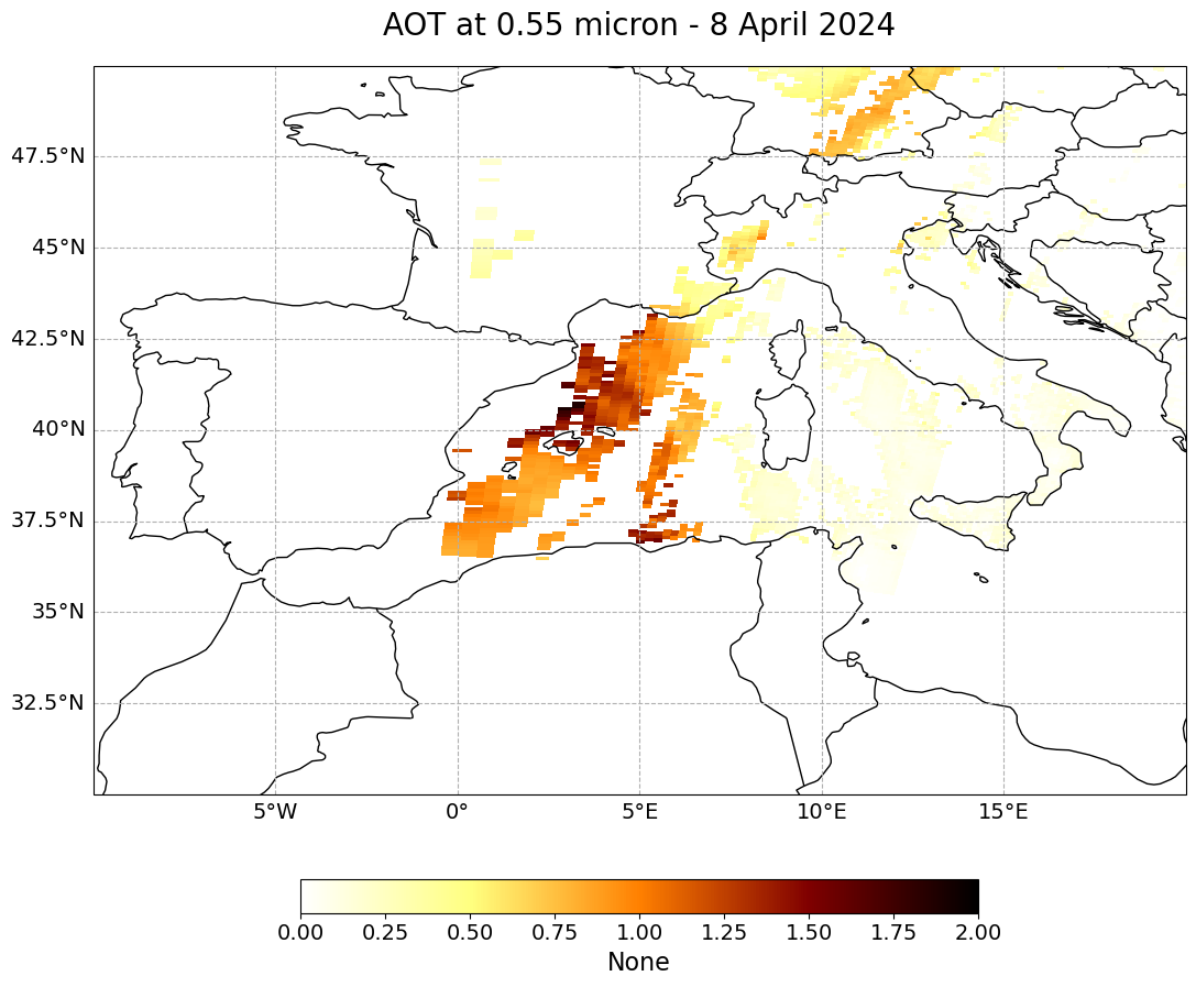
Visualize ‘Optical_Depth_Land_And_Ocean’ over the Mediterranean#
The next step is to visualize the dataset. You can use the function visualize_pcolormesh, which makes use of matploblib’s function pcolormesh and the Cartopy library.
With ?visualize_pcolormesh you can open the function’s docstring to see what keyword arguments are needed to prepare your plot.
?visualize_pcolormesh
You can make use of the variables we have defined above:
long_namelatitudelongitudeunits
Additionally, you can specify the color scale and minimum and maximum data values.
visualize_pcolormesh(data_array=data,
                     longitude=longitude,
                     latitude=latitude,
                     projection=ccrs.PlateCarree(),
                     color_scale='afmhot_r',
                     unit=units,
                     long_name=long_name[0:19] + "- 8 April 2024",
                     vmin=0,
                     vmax=2,
                     lonmin=-10,
                     lonmax=20,
                     latmin=30,
                     latmax=50,
                     set_global=False)
(<Figure size 2000x1000 with 2 Axes>,
 <GeoAxes: title={'center': 'AOT at 0.55 micron - 8 April 2024'}>)