EARLINET Lidar backscatter profiles#
The European Aerosol Research Lidar Network (EARLINET), was established in 2000 as a research project with the goal of creating a quantitative, comprehensive, and statistically significant database for the horizontal, vertical, and temporal distribution of aerosols on a continental scale. Since then EARLINET has continued to provide the most extensive collection of ground-based data for the aerosol vertical distribution over Europe.
Atmospheric aerosols are considered one of the major uncertainties in climate forcing, and a detailed aerosol characterization is needed in order to understand their role in the atmospheric processes as well as human health and environment. The most significant source of uncertainty is the large variability in space and time. Due to their short lifetime and strong interactions, their global concentrations and properties are poorly known. For these reasons, information on the large-scale three-dimensional aerosol distribution in the atmosphere should be continuously monitored. It is undoubted that information on the vertical distribution is particularly important and that lidar remote sensing is the most appropriate tool for providing this information.
EARLINET offers access to long-term multi-wavelength backscatter and extinction coefficient profiles via an easily accessible database, covering the European continent. See here an overview of the EARLINET Lidar Stations.
Basic facts
Spatial coverage: Observation stations in Europe
Temporal resolution: sub-hourly
Temporal coverage: since 2000
Data format: NetCDF
Versions: Level 1 (basic quality control), Level 2 (advanced quality control), Level 3 (climatological aggregated products)
How to access the data
EARLINET data are available in netCDF and can be accessed via the EARLINET Database. Data are offered on different quality controlled levels:
Level 1: Basic quality controlLevel 2: Advanced quality control, andLevel 3: Climatological aggregated products
For the example below, we selected data on 23 February 2021 for the station IPR, which stands for Ispra, Italy, with the following characteristics:
Emission wavelengths:
1064File Types:
b - BackscatterLevels:
Level 2.0
When you click on SEARCH FILES, you get an overview of all available files with the selected characteristics. The files are disseminated in netCDF format.
Note: You have to register for the EARLINET Data Portal in order to be able to download EARLINET data.
Load required libraries
import pandas as pd
import xarray as xr

import matplotlib.pyplot as plt
Load and browse EARLINET data with xarray#
EARLINET data are disseminated as hourly files in the NetCDF format. You can use the Python package xarray and the function open_mfdataset() to open multiple NetCDF at once. Let us load the data files for the EARLINET station Ispra, Italy for 23 February 2021. (NOTE: EARLINET data are not available fore every station and day. Hence, this notebook showcases a case study of a Saharan dust event in Europe that occurred in February 2021).
The function loads the data as Dataset, which is a collection of multiple data variables that share the same coordinate information. Below, you see that the EARLINET data have four dimensions: altitude, time, nv and wavelength.
The data also hold 27 data variables, including a variable backscatter, which is the variable of interest for us.
file_dir = '../../eodata/2_observations/earlinet/Level2/ipr/0223/'
earlinet_2302 = xr.open_mfdataset(file_dir+'*')
earlinet_2302
<xarray.Dataset>
Dimensions:                                         (altitude: 128, nv: 2, time: 9, wavelength: 1)
Coordinates:
  * altitude                                        (altitude) float64 539.0 ...
  * time                                            (time) datetime64[ns] 202...
  * wavelength                                      (wavelength) float32 1.06...
    longitude                                       float32 8.617
    latitude                                        float32 45.82
Dimensions without coordinates: nv
Data variables:
    time_bounds                                     (altitude, time, nv) datetime64[ns] dask.array<chunksize=(128, 1, 2), meta=np.ndarray>
    backscatter_calibration_value                   (time, altitude, wavelength) float32 dask.array<chunksize=(1, 128, 1), meta=np.ndarray>
    error_retrieval_method                          (time, altitude, wavelength) float32 dask.array<chunksize=(1, 128, 1), meta=np.ndarray>
    backscatter_evaluation_method                   (time, altitude, wavelength) float32 dask.array<chunksize=(1, 128, 1), meta=np.ndarray>
    backscatter_calibration_range_search_algorithm  (time, altitude, wavelength) float32 dask.array<chunksize=(1, 128, 1), meta=np.ndarray>
    elastic_backscatter_algorithm                   (time, altitude, wavelength) float32 dask.array<chunksize=(1, 128, 1), meta=np.ndarray>
    station_altitude                                (time, altitude) float64 ...
    zenith_angle                                    (time, altitude) float64 ...
    shots                                           (altitude, time) float64 dask.array<chunksize=(128, 1), meta=np.ndarray>
    atmospheric_molecular_calculation_source        (time, altitude) float64 ...
    cirrus_contamination                            (time, altitude) float64 ...
    cirrus_contamination_source                     (time, altitude) float64 ...
    quality_control_level                           (time, altitude) float64 ...
    basic_quality_control                           (time, altitude) float64 ...
    advanced_quality_control                        (time, altitude) float64 ...
    backscatter                                     (wavelength, time, altitude) float64 dask.array<chunksize=(1, 1, 128), meta=np.ndarray>
    error_backscatter                               (wavelength, time, altitude) float64 dask.array<chunksize=(1, 1, 128), meta=np.ndarray>
    vertical_resolution                             (wavelength, time, altitude) float64 dask.array<chunksize=(1, 1, 128), meta=np.ndarray>
    assumed_particle_lidar_ratio                    (wavelength, time, altitude) float64 dask.array<chunksize=(1, 1, 128), meta=np.ndarray>
    assumed_particle_lidar_ratio_error              (wavelength, time, altitude) float64 dask.array<chunksize=(1, 1, 128), meta=np.ndarray>
    earlinet_product_type                           (time, altitude) float64 ...
    user_defined_category                           (time, altitude) float64 ...
    backscatter_calibration_range                   (time, altitude, wavelength, nv) float32 dask.array<chunksize=(1, 128, 1, 2), meta=np.ndarray>
    backscatter_calibration_search_range            (time, altitude, wavelength, nv) float32 dask.array<chunksize=(1, 128, 1, 2), meta=np.ndarray>
    cloud_mask_type                                 (time, altitude) float64 ...
    scc_product_type                                (time, altitude) float64 ...
    cloud_mask                                      (time, altitude) float32 dask.array<chunksize=(1, 128), meta=np.ndarray>
Attributes:
    Conventions:                          CF-1.7
    title:                                Profiles of aerosol optical properties
    source:                               Ground based LIDAR measurements
    references:                           Project website at http://www.earli...
    history:                              2021-10-06T09:20Z : Assigned versio...
    station_ID:                           ipr
    location:                             Ispra, Italy
    system:                               ADAM-noew-2019
    institution:                          Joint Research Centre - Institute f...
    comment:
    measurement_ID:                       20210223is10
    measurement_start_datetime:           2021-02-23T11:02:16Z
    measurement_stop_datetime:            2021-02-23T11:29:18Z
    PI:                                   Jean Putaud
    PI_affiliation:                       Joint Research Centre - Air and Cli...
    PI_affiliation_acronym:               JRC
    PI_address:
    PI_phone:                             +39 0332 78 50 41
    PI_email:                             jean.putaud@ec.europa.eu
    Data_Originator:                      jean.putaud
    Data_Originator_affiliation:          Joint Research Centre
    Data_Originator_affiliation_acronym:  JRC
    Data_Originator_address:              21027 Ispra (VA)
    Data_Originator_phone:                ++390332785041
    Data_Originator_email:                jean.putaud@ec.europa.eu
    data_processing_institution:          Consiglio Nazionale delle Ricerche ...
    hoi_system_ID:                        164
    hoi_configuration_ID:                 551
    scc_version:                          5.2.3
    scc_version_description:              SCC vers. 5.2.3 (HiRELPP vers. 1.1....
    processor_name:                       ELDA
    processor_version:                    3.4.8
    __file_format_version:                2.1
    input_file:                           ipr_003_0000753_202102231102_202102...
overlap_correction_file: - altitude: 128
- nv: 2
- time: 9
- wavelength: 1
- altitude(altitude)float64539.0 599.0 ... 8.099e+03 8.159e+03
- axis :
- Z
- long_name :
- height above sea level
- positive :
- up
- standard_name :
- altitude
- units :
- m
array([ 539., 599., 659., 719., 779., 839., 899., 959., 1019., 1079., 1139., 1199., 1259., 1319., 1379., 1439., 1499., 1559., 1619., 1679., 1739., 1799., 1859., 1919., 1979., 2039., 2099., 2159., 2219., 2279., 2339., 2399., 2459., 2519., 2579., 2639., 2699., 2759., 2819., 2879., 2939., 2999., 3059., 3119., 3179., 3239., 3299., 3359., 3419., 3479., 3539., 3599., 3659., 3719., 3779., 3839., 3899., 3959., 4019., 4079., 4139., 4199., 4259., 4319., 4379., 4439., 4499., 4559., 4619., 4679., 4739., 4799., 4859., 4919., 4979., 5039., 5099., 5159., 5219., 5279., 5339., 5399., 5459., 5519., 5579., 5639., 5699., 5759., 5819., 5879., 5939., 5999., 6059., 6119., 6179., 6239., 6299., 6359., 6419., 6479., 6539., 6599., 6659., 6719., 6779., 6839., 6899., 6959., 7019., 7079., 7139., 7199., 7259., 7319., 7379., 7439., 7499., 7559., 7619., 7679., 7739., 7799., 7859., 7919., 7979., 8039., 8099., 8159.]) - time(time)datetime64[ns]2021-02-23T11:02:16 ... 2021-02-...
- axis :
- T
- bounds :
- time_bounds
- long_name :
- time
- standard_name :
- time
array(['2021-02-23T11:02:16.000000000', '2021-02-23T12:00:22.999999744', '2021-02-23T12:59:28.000000000', '2021-02-23T14:01:25.999999744', '2021-02-23T15:00:31.000000512', '2021-02-23T16:01:30.999999744', '2021-02-23T17:54:29.999999488', '2021-02-23T18:53:35.000000512', '2021-02-23T19:45:28.000000256'], dtype='datetime64[ns]') - wavelength(wavelength)float321.064e+03
- long_name :
- wavelength of the transmitted laser pulse
- units :
- nm
array([1064.], dtype=float32)
- longitude()float328.617
- long_name :
- longitude of station
- standard_name :
- longitude
- units :
- degrees_east
array(8.6167, dtype=float32)
- latitude()float3245.82
- long_name :
- latitude of station
- standard_name :
- latitude
- units :
- degrees_north
array(45.8167, dtype=float32)
- time_bounds(altitude, time, nv)datetime64[ns]dask.array<chunksize=(128, 1, 2), meta=np.ndarray>
Array Chunk Bytes 18.00 kiB 2.00 kiB Shape (128, 9, 2) (128, 1, 2) Count 91 Tasks 9 Chunks Type datetime64[ns] numpy.ndarray - backscatter_calibration_value(time, altitude, wavelength)float32dask.array<chunksize=(1, 128, 1), meta=np.ndarray>
- long_name :
- assumed backscatter-ratio value in calibration range
- units :
- m-1*sr-1
Array Chunk Bytes 4.50 kiB 512 B Shape (9, 128, 1) (1, 128, 1) Count 91 Tasks 9 Chunks Type float32 numpy.ndarray - error_retrieval_method(time, altitude, wavelength)float32dask.array<chunksize=(1, 128, 1), meta=np.ndarray>
- long_name :
- method used for the retrieval of uncertainties
- flag_values :
- [0 1]
- flag_meanings :
- monte_carlo error_propagation
Array Chunk Bytes 4.50 kiB 512 B Shape (9, 128, 1) (1, 128, 1) Count 91 Tasks 9 Chunks Type float32 numpy.ndarray - backscatter_evaluation_method(time, altitude, wavelength)float32dask.array<chunksize=(1, 128, 1), meta=np.ndarray>
- long_name :
- method used for the backscatter retrieval
- flag_values :
- [0 1]
- flag_meanings :
- Raman elastic_backscatter
Array Chunk Bytes 4.50 kiB 512 B Shape (9, 128, 1) (1, 128, 1) Count 91 Tasks 9 Chunks Type float32 numpy.ndarray - backscatter_calibration_range_search_algorithm(time, altitude, wavelength)float32dask.array<chunksize=(1, 128, 1), meta=np.ndarray>
- long_name :
- algorithm used for the search of the calibration_range
- flag_values :
- [0 1]
- flag_meanings :
- minimum_of_signal_ratio minimum_of_elastic_signal
Array Chunk Bytes 4.50 kiB 512 B Shape (9, 128, 1) (1, 128, 1) Count 91 Tasks 9 Chunks Type float32 numpy.ndarray - elastic_backscatter_algorithm(time, altitude, wavelength)float32dask.array<chunksize=(1, 128, 1), meta=np.ndarray>
- long_name :
- 0: Klett-Fernald, 1: iterative
- flag_values :
- [0 1]
- flag_meanings :
- Klett-Fernald iterative
Array Chunk Bytes 4.50 kiB 512 B Shape (9, 128, 1) (1, 128, 1) Count 91 Tasks 9 Chunks Type float32 numpy.ndarray - station_altitude(time, altitude)float64209.0 209.0 209.0 ... nan nan nan
- long_name :
- station altitude above see level
- units :
- m
array([[209., 209., 209., ..., nan, nan, nan], [209., 209., 209., ..., nan, nan, nan], [209., 209., 209., ..., nan, nan, nan], ..., [209., 209., 209., ..., 209., 209., 209.], [209., 209., 209., ..., nan, nan, nan], [209., 209., 209., ..., nan, nan, nan]]) - zenith_angle(time, altitude)float640.0 0.0 0.0 0.0 ... nan nan nan nan
- long_name :
- laser pointing angle with respect to the zenith
- units :
- degrees
array([[ 0., 0., 0., ..., nan, nan, nan], [ 0., 0., 0., ..., nan, nan, nan], [ 0., 0., 0., ..., nan, nan, nan], ..., [ 0., 0., 0., ..., 0., 0., 0.], [ 0., 0., 0., ..., nan, nan, nan], [ 0., 0., 0., ..., nan, nan, nan]]) - shots(altitude, time)float64dask.array<chunksize=(128, 1), meta=np.ndarray>
- long_name :
- accumulated laser shots
- units :
- 1
Array Chunk Bytes 9.00 kiB 1.00 kiB Shape (128, 9) (128, 1) Count 82 Tasks 9 Chunks Type float64 numpy.ndarray - atmospheric_molecular_calculation_source(time, altitude)float646.0 6.0 6.0 6.0 ... nan nan nan nan
- long_name :
- data source of the atmospheric molecular calculations
- valid_range :
- [0 8]
- flag_values :
- [0 1 2 3 4 5 6 7 8]
- flag_meanings :
- US_standard_atmosphere radiosounding ecmwf icon_iglo_12_23 icon_iglo_24_35 icon_iglo_36_47 gdas era5-1-12 era5-7-18
array([[ 6., 6., 6., ..., nan, nan, nan], [ 6., 6., 6., ..., nan, nan, nan], [ 6., 6., 6., ..., nan, nan, nan], ..., [ 6., 6., 6., ..., 6., 6., 6.], [ 6., 6., 6., ..., nan, nan, nan], [ 6., 6., 6., ..., nan, nan, nan]]) - cirrus_contamination(time, altitude)float641.0 1.0 1.0 1.0 ... nan nan nan nan
- long_name :
- do the profiles contain cirrus layers?
- valid_range :
- [0 3]
- flag_values :
- [0 1 2]
- flag_meanings :
- not_available no_cirrus cirrus_detected
array([[ 1., 1., 1., ..., nan, nan, nan], [ 1., 1., 1., ..., nan, nan, nan], [ 1., 1., 1., ..., nan, nan, nan], ..., [ 1., 1., 1., ..., 1., 1., 1.], [ 1., 1., 1., ..., nan, nan, nan], [ 1., 1., 1., ..., nan, nan, nan]]) - cirrus_contamination_source(time, altitude)float642.0 2.0 2.0 2.0 ... nan nan nan nan
- long_name :
- how was cirrus_contamination obtained?
- valid_range :
- [0 3]
- flag_values :
- [0 1 2]
- flag_meanings :
- not_available user_provided automatic_calculated
array([[ 2., 2., 2., ..., nan, nan, nan], [ 2., 2., 2., ..., nan, nan, nan], [ 2., 2., 2., ..., nan, nan, nan], ..., [ 2., 2., 2., ..., 2., 2., 2.], [ 2., 2., 2., ..., nan, nan, nan], [ 2., 2., 2., ..., nan, nan, nan]]) - quality_control_level(time, altitude)float642.0 2.0 2.0 2.0 ... nan nan nan nan
- long_name :
- Quality Control Level
- flag_values :
- [0 1 2]
- flag_meanings :
- File_does_not_overcome_one_or_more_on_fly_quality_control File_does_overcome_all_on_fly_quality_control_but_fails_one_or_more_technical_quality_control File_does_overcome_all_technical_quality_control_and_physical_quality_control
- version :
- 2.0
- references :
- https://www.earlinet.org/index.php?id=293
array([[ 2., 2., 2., ..., nan, nan, nan], [ 2., 2., 2., ..., nan, nan, nan], [ 2., 2., 2., ..., nan, nan, nan], ..., [ 2., 2., 2., ..., 2., 2., 2.], [ 2., 2., 2., ..., nan, nan, nan], [ 2., 2., 2., ..., nan, nan, nan]]) - basic_quality_control(time, altitude)float647.0 7.0 7.0 7.0 ... nan nan nan nan
- long_name :
- Basic Quality Control
- valid_range :
- [0 7]
- flag_masks :
- [1 2 4]
- flag_meanings :
- Check_if_file_contains_data Check_Coordinates_Consistency Check_for_Undefined_Variables_and_Global_Attributes
- references :
- https://www.earlinet.org/index.php?id=293
array([[ 7., 7., 7., ..., nan, nan, nan], [ 7., 7., 7., ..., nan, nan, nan], [ 7., 7., 7., ..., nan, nan, nan], ..., [ 7., 7., 7., ..., 7., 7., 7.], [ 7., 7., 7., ..., nan, nan, nan], [ 7., 7., 7., ..., nan, nan, nan]]) - advanced_quality_control(time, altitude)float642.027e+03 2.027e+03 ... nan nan
- long_name :
- Advanced Quality Control
- valid_range :
- [ 0 2027]
- flag_masks :
- [ 1 2 8 32 64 128 256 512 1024]
- flag_meanings :
- Checks_for_Negative_Errors Negative_peaks Check_on_IB Check_on_Volumedepolarization Check_on_Particledepolarization Check_on_Watervapormixingratio Check_on_atmospheric_molecular_calculation_source Check_on_old_cirrus_product Check_on_SCC_product_type
- references :
- https://www.earlinet.org/index.php?id=293
array([[2027., 2027., 2027., ..., nan, nan, nan], [2027., 2027., 2027., ..., nan, nan, nan], [2027., 2027., 2027., ..., nan, nan, nan], ..., [2027., 2027., 2027., ..., 2027., 2027., 2027.], [2027., 2027., 2027., ..., nan, nan, nan], [2027., 2027., 2027., ..., nan, nan, nan]]) - backscatter(wavelength, time, altitude)float64dask.array<chunksize=(1, 1, 128), meta=np.ndarray>
- ancillary_variables :
- error_backscatter vertical_resolution
- long_name :
- aerosol backscatter coefficient
- plausibility :
- parameter passed the EARLINET quality assurance.
- units :
- m-1*sr-1
Array Chunk Bytes 9.00 kiB 1.00 kiB Shape (1, 9, 128) (1, 1, 128) Count 74 Tasks 9 Chunks Type float64 numpy.ndarray - error_backscatter(wavelength, time, altitude)float64dask.array<chunksize=(1, 1, 128), meta=np.ndarray>
- long_name :
- statistical uncertainty of aerosol backscatter
- plausibility :
- parameter passed the EARLINET quality assurance.
- units :
- m-1*sr-1
Array Chunk Bytes 9.00 kiB 1.00 kiB Shape (1, 9, 128) (1, 1, 128) Count 74 Tasks 9 Chunks Type float64 numpy.ndarray - vertical_resolution(wavelength, time, altitude)float64dask.array<chunksize=(1, 1, 128), meta=np.ndarray>
- long_name :
- effective vertical resolution according to Pappalardo et al., appl. opt. 2004
- units :
- m
Array Chunk Bytes 9.00 kiB 1.00 kiB Shape (1, 9, 128) (1, 1, 128) Count 74 Tasks 9 Chunks Type float64 numpy.ndarray - assumed_particle_lidar_ratio(wavelength, time, altitude)float64dask.array<chunksize=(1, 1, 128), meta=np.ndarray>
- long_name :
- assumed particle lidar ratio value to use in elastic only backscatter retrieval
- units :
- sr
Array Chunk Bytes 9.00 kiB 1.00 kiB Shape (1, 9, 128) (1, 1, 128) Count 74 Tasks 9 Chunks Type float64 numpy.ndarray - assumed_particle_lidar_ratio_error(wavelength, time, altitude)float64dask.array<chunksize=(1, 1, 128), meta=np.ndarray>
- long_name :
- assumed_particle_lidar_ratio_error
- units :
- sr
Array Chunk Bytes 9.00 kiB 1.00 kiB Shape (1, 9, 128) (1, 1, 128) Count 74 Tasks 9 Chunks Type float64 numpy.ndarray - earlinet_product_type(time, altitude)float648.0 8.0 8.0 8.0 ... nan nan nan nan
- long_name :
- Earlinet product type
- valid_range :
- [ 1 14]
- flag_values :
- [ 1 2 3 4 5 6 7 8 9 10 11 12 13 14]
- flag_meanings :
- e0355 b0355 e0351 b0351 e0532 b0532 e1064 b1064 b0253 b0313 b0335 b0510 b0694 b0817
array([[ 8., 8., 8., ..., nan, nan, nan], [ 8., 8., 8., ..., nan, nan, nan], [ 8., 8., 8., ..., nan, nan, nan], ..., [ 8., 8., 8., ..., 8., 8., 8.], [ 8., 8., 8., ..., nan, nan, nan], [ 8., 8., 8., ..., nan, nan, nan]]) - user_defined_category(time, altitude)float640.0 0.0 0.0 0.0 ... nan nan nan nan
- long_name :
- User defined category of the measurement
- valid_range :
- [ 0 1023]
- flag_masks :
- [ 1 2 4 8 16 32 64 128 256 512]
- flag_meanings :
- cirrus climatology diurnal_cycles volcanic forest_fires photosmog rural_urban saharan_dust stratosphere satellite_overpasses
- comment :
- Those flags might have not been set in a homogeneous way. Before using them, contact the originator to obtain more detailed information on how these flags have been set.
array([[ 0., 0., 0., ..., nan, nan, nan], [ 0., 0., 0., ..., nan, nan, nan], [ 0., 0., 0., ..., nan, nan, nan], ..., [ 0., 0., 0., ..., 0., 0., 0.], [ 0., 0., 0., ..., nan, nan, nan], [ 0., 0., 0., ..., nan, nan, nan]]) - backscatter_calibration_range(time, altitude, wavelength, nv)float32dask.array<chunksize=(1, 128, 1, 2), meta=np.ndarray>
- long_name :
- altitude range where calibration was calculated
- units :
- m
Array Chunk Bytes 9.00 kiB 1.00 kiB Shape (9, 128, 1, 2) (1, 128, 1, 2) Count 100 Tasks 9 Chunks Type float32 numpy.ndarray - backscatter_calibration_search_range(time, altitude, wavelength, nv)float32dask.array<chunksize=(1, 128, 1, 2), meta=np.ndarray>
- long_name :
- altitude range wherein calibration range is searched
- units :
- m
Array Chunk Bytes 9.00 kiB 1.00 kiB Shape (9, 128, 1, 2) (1, 128, 1, 2) Count 100 Tasks 9 Chunks Type float32 numpy.ndarray - cloud_mask_type(time, altitude)float642.0 2.0 2.0 2.0 ... nan nan nan nan
- long_name :
- cloud mask type
- valid_range :
- [0 3]
- flag_values :
- [0 1 2]
- flag_meanings :
- no_cloudmask_available manual_cloudmask automatic_cloudmask
array([[ 2., 2., 2., ..., nan, nan, nan], [ 2., 2., 2., ..., nan, nan, nan], [ 2., 2., 2., ..., nan, nan, nan], ..., [ 2., 2., 2., ..., 2., 2., 2.], [ 2., 2., 2., ..., nan, nan, nan], [ 2., 2., 2., ..., nan, nan, nan]]) - scc_product_type(time, altitude)float641.0 1.0 1.0 1.0 ... nan nan nan nan
- long_name :
- SCC product type
- valid_range :
- [1 2]
- flag_values :
- [1 2]
- flag_meanings :
- experimental operational
array([[ 1., 1., 1., ..., nan, nan, nan], [ 1., 1., 1., ..., nan, nan, nan], [ 1., 1., 1., ..., nan, nan, nan], ..., [ 1., 1., 1., ..., 1., 1., 1.], [ 1., 1., 1., ..., nan, nan, nan], [ 1., 1., 1., ..., nan, nan, nan]]) - cloud_mask(time, altitude)float32dask.array<chunksize=(1, 128), meta=np.ndarray>
- long_name :
- cloud mask
- valid_range :
- [0 7]
- flag_masks :
- [1 2 4]
- flag_meanings :
- unknown_cloud cirrus_cloud water_cloud
Array Chunk Bytes 4.50 kiB 512 B Shape (9, 128) (1, 128) Count 73 Tasks 9 Chunks Type float32 numpy.ndarray
- Conventions :
- CF-1.7
- title :
- Profiles of aerosol optical properties
- source :
- Ground based LIDAR measurements
- references :
- Project website at http://www.earlinet.org
- history :
- 2021-10-06T09:20Z : Assigned version 1 2021-10-06T09:20:00Z : File uploaded on Earlinet database 2021-10-04T13:09:57Z: elpp -d sccoperational -m 20210223is10 -c elpp.config; 2021-10-04T13:10:26Z: elda 20210223is10 -c elda.ini
- station_ID :
- ipr
- location :
- Ispra, Italy
- system :
- ADAM-noew-2019
- institution :
- Joint Research Centre - Institute for Environment and Sustainability, Ispra - JRC
- comment :
- measurement_ID :
- 20210223is10
- measurement_start_datetime :
- 2021-02-23T11:02:16Z
- measurement_stop_datetime :
- 2021-02-23T11:29:18Z
- PI :
- Jean Putaud
- PI_affiliation :
- Joint Research Centre - Air and Climate Unit, Ispra
- PI_affiliation_acronym :
- JRC
- PI_address :
- PI_phone :
- +39 0332 78 50 41
- PI_email :
- jean.putaud@ec.europa.eu
- Data_Originator :
- jean.putaud
- Data_Originator_affiliation :
- Joint Research Centre
- Data_Originator_affiliation_acronym :
- JRC
- Data_Originator_address :
- 21027 Ispra (VA)
- Data_Originator_phone :
- ++390332785041
- Data_Originator_email :
- jean.putaud@ec.europa.eu
- data_processing_institution :
- Consiglio Nazionale delle Ricerche - Istituto di Metodologie per l'Analisi Ambientale (CNR-IMAA)
- hoi_system_ID :
- 164
- hoi_configuration_ID :
- 551
- scc_version :
- 5.2.3
- scc_version_description :
- SCC vers. 5.2.3 (HiRELPP vers. 1.1.2, CloudMask vers. 1.6.0, ELPP vers. 7.1.3, ELDA vers. 3.4.8, ELIC vers. 1.0.7, ELQUICK vers. 1.0.7, ELDEC vers. 2.1.3)
- processor_name :
- ELDA
- processor_version :
- 3.4.8
- __file_format_version :
- 2.1
- input_file :
- ipr_003_0000753_202102231102_202102231129_20210223is10_elpp_v5.2.3.nc
- overlap_correction_file :
EARLINET Lidar sensors create vertical profiles of the atmosphere. Let us inspect the variable altitude in order to see the resolution and extent of the vertical profile. You see that the EARLINET data offer measurements for every 40 meters from 539 m up to 8 km.
earlinet_2302.altitude
<xarray.DataArray 'altitude' (altitude: 128)>
array([ 539.,  599.,  659.,  719.,  779.,  839.,  899.,  959., 1019., 1079.,
       1139., 1199., 1259., 1319., 1379., 1439., 1499., 1559., 1619., 1679.,
       1739., 1799., 1859., 1919., 1979., 2039., 2099., 2159., 2219., 2279.,
       2339., 2399., 2459., 2519., 2579., 2639., 2699., 2759., 2819., 2879.,
       2939., 2999., 3059., 3119., 3179., 3239., 3299., 3359., 3419., 3479.,
       3539., 3599., 3659., 3719., 3779., 3839., 3899., 3959., 4019., 4079.,
       4139., 4199., 4259., 4319., 4379., 4439., 4499., 4559., 4619., 4679.,
       4739., 4799., 4859., 4919., 4979., 5039., 5099., 5159., 5219., 5279.,
       5339., 5399., 5459., 5519., 5579., 5639., 5699., 5759., 5819., 5879.,
       5939., 5999., 6059., 6119., 6179., 6239., 6299., 6359., 6419., 6479.,
       6539., 6599., 6659., 6719., 6779., 6839., 6899., 6959., 7019., 7079.,
       7139., 7199., 7259., 7319., 7379., 7439., 7499., 7559., 7619., 7679.,
       7739., 7799., 7859., 7919., 7979., 8039., 8099., 8159.])
Coordinates:
  * altitude   (altitude) float64 539.0 599.0 659.0 ... 8.099e+03 8.159e+03
    longitude  float32 8.617
    latitude   float32 45.82
Attributes:
    axis:           Z
    long_name:      height above sea level
    positive:       up
    standard_name:  altitude
units: m- altitude: 128
- 539.0 599.0 659.0 719.0 ... 7.979e+03 8.039e+03 8.099e+03 8.159e+03
array([ 539., 599., 659., 719., 779., 839., 899., 959., 1019., 1079., 1139., 1199., 1259., 1319., 1379., 1439., 1499., 1559., 1619., 1679., 1739., 1799., 1859., 1919., 1979., 2039., 2099., 2159., 2219., 2279., 2339., 2399., 2459., 2519., 2579., 2639., 2699., 2759., 2819., 2879., 2939., 2999., 3059., 3119., 3179., 3239., 3299., 3359., 3419., 3479., 3539., 3599., 3659., 3719., 3779., 3839., 3899., 3959., 4019., 4079., 4139., 4199., 4259., 4319., 4379., 4439., 4499., 4559., 4619., 4679., 4739., 4799., 4859., 4919., 4979., 5039., 5099., 5159., 5219., 5279., 5339., 5399., 5459., 5519., 5579., 5639., 5699., 5759., 5819., 5879., 5939., 5999., 6059., 6119., 6179., 6239., 6299., 6359., 6419., 6479., 6539., 6599., 6659., 6719., 6779., 6839., 6899., 6959., 7019., 7079., 7139., 7199., 7259., 7319., 7379., 7439., 7499., 7559., 7619., 7679., 7739., 7799., 7859., 7919., 7979., 8039., 8099., 8159.]) - altitude(altitude)float64539.0 599.0 ... 8.099e+03 8.159e+03
- axis :
- Z
- long_name :
- height above sea level
- positive :
- up
- standard_name :
- altitude
- units :
- m
array([ 539., 599., 659., 719., 779., 839., 899., 959., 1019., 1079., 1139., 1199., 1259., 1319., 1379., 1439., 1499., 1559., 1619., 1679., 1739., 1799., 1859., 1919., 1979., 2039., 2099., 2159., 2219., 2279., 2339., 2399., 2459., 2519., 2579., 2639., 2699., 2759., 2819., 2879., 2939., 2999., 3059., 3119., 3179., 3239., 3299., 3359., 3419., 3479., 3539., 3599., 3659., 3719., 3779., 3839., 3899., 3959., 4019., 4079., 4139., 4199., 4259., 4319., 4379., 4439., 4499., 4559., 4619., 4679., 4739., 4799., 4859., 4919., 4979., 5039., 5099., 5159., 5219., 5279., 5339., 5399., 5459., 5519., 5579., 5639., 5699., 5759., 5819., 5879., 5939., 5999., 6059., 6119., 6179., 6239., 6299., 6359., 6419., 6479., 6539., 6599., 6659., 6719., 6779., 6839., 6899., 6959., 7019., 7079., 7139., 7199., 7259., 7319., 7379., 7439., 7499., 7559., 7619., 7679., 7739., 7799., 7859., 7919., 7979., 8039., 8099., 8159.]) - longitude()float328.617
- long_name :
- longitude of station
- standard_name :
- longitude
- units :
- degrees_east
array(8.6167, dtype=float32)
- latitude()float3245.82
- long_name :
- latitude of station
- standard_name :
- latitude
- units :
- degrees_north
array(45.8167, dtype=float32)
- axis :
- Z
- long_name :
- height above sea level
- positive :
- up
- standard_name :
- altitude
- units :
- m
As a last step before we can visualize the vertical profile, we can load the variable backscatter from the dataset. You can load a variable from a xarray.Dataset by adding the name of the variable in square brackets.
The loaded data array provides you additional attributes about the data, such as long_name and units.
backscatter = earlinet_2302['backscatter']
backscatter
<xarray.DataArray 'backscatter' (wavelength: 1, time: 9, altitude: 128)>
dask.array<concatenate, shape=(1, 9, 128), dtype=float64, chunksize=(1, 1, 128), chunktype=numpy.ndarray>
Coordinates:
  * altitude    (altitude) float64 539.0 599.0 659.0 ... 8.099e+03 8.159e+03
  * time        (time) datetime64[ns] 2021-02-23T11:02:16 ... 2021-02-23T19:4...
  * wavelength  (wavelength) float32 1.064e+03
    longitude   float32 8.617
    latitude    float32 45.82
Attributes:
    ancillary_variables:  error_backscatter vertical_resolution
    long_name:            aerosol backscatter coefficient
    plausibility:         parameter passed the EARLINET quality assurance.
units: m-1*sr-1- wavelength: 1
- time: 9
- altitude: 128
- dask.array<chunksize=(1, 1, 128), meta=np.ndarray>
Array Chunk Bytes 9.22 kB 1.02 kB Shape (1, 9, 128) (1, 1, 128) Count 74 Tasks 9 Chunks Type float64 numpy.ndarray - altitude(altitude)float64539.0 599.0 ... 8.099e+03 8.159e+03
- axis :
- Z
- long_name :
- height above sea level
- positive :
- up
- standard_name :
- altitude
- units :
- m
array([ 539., 599., 659., 719., 779., 839., 899., 959., 1019., 1079., 1139., 1199., 1259., 1319., 1379., 1439., 1499., 1559., 1619., 1679., 1739., 1799., 1859., 1919., 1979., 2039., 2099., 2159., 2219., 2279., 2339., 2399., 2459., 2519., 2579., 2639., 2699., 2759., 2819., 2879., 2939., 2999., 3059., 3119., 3179., 3239., 3299., 3359., 3419., 3479., 3539., 3599., 3659., 3719., 3779., 3839., 3899., 3959., 4019., 4079., 4139., 4199., 4259., 4319., 4379., 4439., 4499., 4559., 4619., 4679., 4739., 4799., 4859., 4919., 4979., 5039., 5099., 5159., 5219., 5279., 5339., 5399., 5459., 5519., 5579., 5639., 5699., 5759., 5819., 5879., 5939., 5999., 6059., 6119., 6179., 6239., 6299., 6359., 6419., 6479., 6539., 6599., 6659., 6719., 6779., 6839., 6899., 6959., 7019., 7079., 7139., 7199., 7259., 7319., 7379., 7439., 7499., 7559., 7619., 7679., 7739., 7799., 7859., 7919., 7979., 8039., 8099., 8159.]) - time(time)datetime64[ns]2021-02-23T11:02:16 ... 2021-02-...
- axis :
- T
- bounds :
- time_bounds
- long_name :
- time
- standard_name :
- time
array(['2021-02-23T11:02:16.000000000', '2021-02-23T12:00:22.999999744', '2021-02-23T12:59:28.000000000', '2021-02-23T14:01:25.999999744', '2021-02-23T15:00:31.000000512', '2021-02-23T16:01:30.999999744', '2021-02-23T17:54:29.999999488', '2021-02-23T18:53:35.000000512', '2021-02-23T19:45:28.000000256'], dtype='datetime64[ns]') - wavelength(wavelength)float321.064e+03
- long_name :
- wavelength of the transmitted laser pulse
- units :
- nm
array([1064.], dtype=float32)
- longitude()float328.617
- long_name :
- longitude of station
- standard_name :
- longitude
- units :
- degrees_east
array(8.6167, dtype=float32)
- latitude()float3245.82
- long_name :
- latitude of station
- standard_name :
- latitude
- units :
- degrees_north
array(45.8167, dtype=float32)
- ancillary_variables :
- error_backscatter vertical_resolution
- long_name :
- aerosol backscatter coefficient
- plausibility :
- parameter passed the EARLINET quality assurance.
- units :
- m-1*sr-1
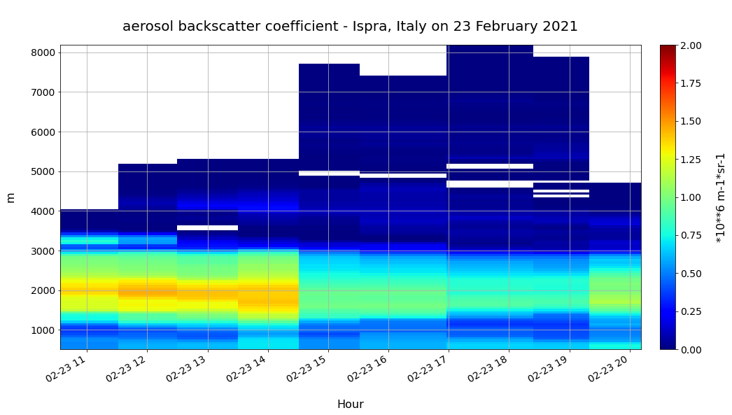
Visualize the backscatter profile in Ispra on 23 February 2021#
Now, we can already visualize the Aerosol backscatter coefficient for the station Ispra on 23 February 2021. We want to plot the time information on the x-axis and the altitude information on the y-axis. The visualization code below can be divided in five main parts:
Initiate a matplotlib figure: Initiate a matplotlib plot and define the size of the plot
Plotting function: plot the xarray.DataArray, but transpose the two dimensions, altitude and time
Set plot title, axes label and format axes tickes: specify title, axes labels and their format
Define and format colorbar: define and customize a colorbar
Add additional features: such as grid lines
# Initiate a matplotlib figure
fig = plt.figure(figsize=(16,8))
ax=plt.axes()

# Plotting function
img = (backscatter*10**6).transpose().plot(vmin=0,
                                             vmax=2,
                                             cmap='jet', ax=ax, add_colorbar=False)

# Set title and axes label information
plt.title('\n' + backscatter.long_name + ' - Ispra, Italy on 23 February 2021', fontsize=20, pad=20)
plt.ylabel(earlinet_2302.altitude.units+'\n', fontsize=16)
plt.xlabel('\nHour', fontsize=16)

# Format the axes ticks
plt.xticks(fontsize=14)
plt.yticks(fontsize=14)

# Define and format colorbar
cbar = fig.colorbar(img, ax=ax, orientation='vertical', fraction=0.04, pad=0.03)
cbar.set_label('\n*10**6 ' + backscatter.units, fontsize=16)
cbar.ax.tick_params(labelsize=14)

# Add additionally a legend and grid to the plot
plt.grid()
Load and visualize backscatter profiles in Ispra for 24+25 Feb 2021#
Let us now also load the backscatter profiles for the station in Ispra for the two following days, 24th and 25th February 2021 respectively. We repeat the same steps as above. First, we load the backscatter profile information as xarray.Dataset with the function open_mfdataset().
Once both datasets are loaded, you see that for 24 February backscatter profiles for four hours are available and for 25 February backscatter profiles for six hours are available.
file_dir = '../../eodata/2_observations/earlinet/Level2/ipr/0224/'
earlinet_2402 = xr.open_mfdataset(file_dir+'*')

file_dir = '../../eodata/2_observations/earlinet/Level2/ipr/0225/'
earlinet_2502 = xr.open_mfdataset(file_dir+'*')

earlinet_2402, earlinet_2502
(<xarray.Dataset>
 Dimensions:                                         (altitude: 82, time: 4, nv: 2, wavelength: 1)
 Coordinates:
   * altitude                                        (altitude) float64 539.0 ...
   * time                                            (time) datetime64[ns] 202...
   * wavelength                                      (wavelength) float32 1.06...
     longitude                                       float32 8.617
     latitude                                        float32 45.82
 Dimensions without coordinates: nv
 Data variables: (12/27)
     time_bounds                                     (altitude, time, nv) datetime64[ns] dask.array<chunksize=(82, 1, 2), meta=np.ndarray>
     backscatter_calibration_value                   (altitude, time, wavelength) float32 dask.array<chunksize=(82, 1, 1), meta=np.ndarray>
     error_retrieval_method                          (altitude, time, wavelength) float32 dask.array<chunksize=(82, 1, 1), meta=np.ndarray>
     backscatter_evaluation_method                   (altitude, time, wavelength) float32 dask.array<chunksize=(82, 1, 1), meta=np.ndarray>
     backscatter_calibration_range_search_algorithm  (altitude, time, wavelength) float32 dask.array<chunksize=(82, 1, 1), meta=np.ndarray>
     elastic_backscatter_algorithm                   (altitude, time, wavelength) float32 dask.array<chunksize=(82, 1, 1), meta=np.ndarray>
     ...                                              ...
     user_defined_category                           (altitude, time) float64 ...
     backscatter_calibration_range                   (altitude, time, wavelength, nv) float32 dask.array<chunksize=(82, 1, 1, 2), meta=np.ndarray>
     backscatter_calibration_search_range            (altitude, time, wavelength, nv) float32 dask.array<chunksize=(82, 1, 1, 2), meta=np.ndarray>
     cloud_mask_type                                 (altitude, time) float64 ...
     scc_product_type                                (altitude, time) float64 ...
     cloud_mask                                      (time, altitude) float32 dask.array<chunksize=(1, 82), meta=np.ndarray>
 Attributes: (12/35)
     Conventions:                          CF-1.7
     title:                                Profiles of aerosol optical properties
     source:                               Ground based LIDAR measurements
     references:                           Project website at http://www.earli...
     history:                              2021-10-06T09:23Z : Assigned versio...
     station_ID:                           ipr
     ...                                   ...
     scc_version_description:              SCC vers. 5.2.3 (HiRELPP vers. 1.1....
     processor_name:                       ELDA
     processor_version:                    3.4.8
     __file_format_version:                2.1
     input_file:                           ipr_003_0000753_202102241406_202102...
     overlap_correction_file:              ,
 <xarray.Dataset>
 Dimensions:                                         (altitude: 84, time: 6, nv: 2, wavelength: 1)
 Coordinates:
   * altitude                                        (altitude) float64 539.0 ...
   * time                                            (time) datetime64[ns] 202...
   * wavelength                                      (wavelength) float32 1.06...
     longitude                                       float32 8.617
     latitude                                        float32 45.82
 Dimensions without coordinates: nv
 Data variables: (12/27)
     time_bounds                                     (altitude, time, nv) datetime64[ns] dask.array<chunksize=(84, 1, 2), meta=np.ndarray>
     backscatter_calibration_value                   (altitude, time, wavelength) float32 dask.array<chunksize=(84, 1, 1), meta=np.ndarray>
     error_retrieval_method                          (altitude, time, wavelength) float32 dask.array<chunksize=(84, 1, 1), meta=np.ndarray>
     backscatter_evaluation_method                   (altitude, time, wavelength) float32 dask.array<chunksize=(84, 1, 1), meta=np.ndarray>
     backscatter_calibration_range_search_algorithm  (altitude, time, wavelength) float32 dask.array<chunksize=(84, 1, 1), meta=np.ndarray>
     elastic_backscatter_algorithm                   (altitude, time, wavelength) float32 dask.array<chunksize=(84, 1, 1), meta=np.ndarray>
     ...                                              ...
     user_defined_category                           (altitude, time) float64 ...
     backscatter_calibration_range                   (altitude, time, wavelength, nv) float32 dask.array<chunksize=(84, 1, 1, 2), meta=np.ndarray>
     backscatter_calibration_search_range            (altitude, time, wavelength, nv) float32 dask.array<chunksize=(84, 1, 1, 2), meta=np.ndarray>
     cloud_mask_type                                 (altitude, time) float64 ...
     scc_product_type                                (altitude, time) float64 ...
     cloud_mask                                      (time, altitude) float32 dask.array<chunksize=(1, 84), meta=np.ndarray>
 Attributes: (12/35)
     Conventions:                          CF-1.7
     title:                                Profiles of aerosol optical properties
     source:                               Ground based LIDAR measurements
     references:                           Project website at http://www.earli...
     history:                              2021-10-06T09:25Z : Assigned versio...
     station_ID:                           ipr
     ...                                   ...
     scc_version_description:              SCC vers. 5.2.3 (HiRELPP vers. 1.1....
     processor_name:                       ELDA
     processor_version:                    3.4.8
     __file_format_version:                2.1
     input_file:                           ipr_003_0000753_202102251123_202102...
     overlap_correction_file:              )
The next step is now to visualize the two backscatter profiles for both days next to each other. We simply replicate the visualization code from above, but create two subplots with with plt.subplot(). By specifying (1,2,1), we create a plot with 1 row and 2 columns and the third number indicates that this is the first plot of two.
# Initiate a matplotlib figure
fig = plt.figure(figsize=(25,8))

########################
# 1st subplot
########################
ax1=plt.subplot(1,2,1)

# Plotting function
img1 = (earlinet_2402['backscatter']*10**6).transpose().plot(vmin=0,
                                             vmax=2,
                                             cmap='jet', ax=ax1, add_colorbar=False)

# Set title and axes label information
plt.title('\n' + earlinet_2402['backscatter'].long_name + ' - Ispra, Italy on 24 February 2021', fontsize=20, pad=20)
plt.ylabel(earlinet_2402.altitude.units+'\n', fontsize=16)
plt.xlabel('\nHour', fontsize=16)

# Format the axes ticks
plt.xticks(fontsize=14)
plt.yticks(fontsize=14)

# Add additionally a legend and grid to the plot
plt.grid()


########################
# 2nd subplot
########################
ax2 = plt.subplot(1,2,2)
# Plotting function
img2 = (earlinet_2502['backscatter']*10**6).transpose().plot(vmin=0,
                                             vmax=2,
                                             cmap='jet', ax=ax2, add_colorbar=False)

# Set title and axes label information
plt.title('\n' + earlinet_2502['backscatter'].long_name + ' - Ispra, Italy on 25 February 2021', fontsize=20, pad=20)
plt.ylabel(earlinet_2502.altitude.units+'\n', fontsize=16)
plt.xlabel('\nHour', fontsize=16)

# Format the axes ticks
plt.xticks(fontsize=14)
plt.yticks(fontsize=14)

# Define and format colorbar
cbar = fig.colorbar(img2, ax=ax2, orientation='vertical', fraction=0.04, pad=0.03)
cbar.set_label('\n*10**6 ' + earlinet_2502['backscatter'].units, fontsize=16)
cbar.ax.tick_params(labelsize=14)

# Add additionally a legend and grid to the plot
plt.grid()
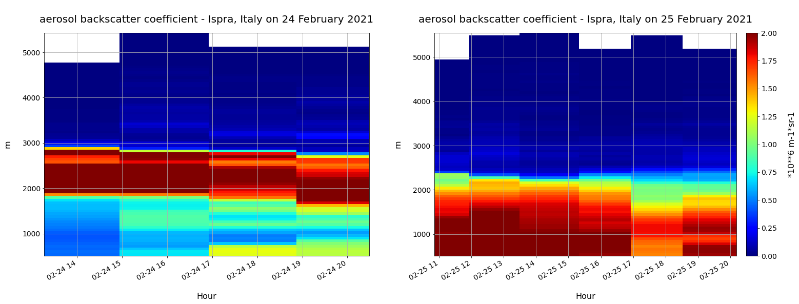
Above, you see that the intensity of the backscatter profile has increased from 23rd to 24th of February, but the aerosol layer was in the upper atmosphere between 2000 and 3000 m above surface. On 25th February, the aerosol layer settled at the surface. This strong aerosol occurence at the surface can also be seen in the EEA Air Qualty data, as the PM10 value exceeded by far the daily limit of 50 µg/m3.