Polar Multi-Sensor Aerosol Optical Properties (PMAp) Product¶

Hint

Execute the notebook on the training platform >>

The following module shows you the structure of PMAp Aerosol Optical Depth Level 2 data and what information of the data files can be used in order to load, browse and visualize Aerosol Optical Depth at 550 nm.

The polar multi-sensor aerosol optical properties product (PMAp) provides information on aerosol optical depth (AOD) at 550 nm and aerosol type (fine mode, coarse mode (dust) and volcanic ash) over ocean and land surfaces. The product is generated based on the Meteosat Second Generation instrument GOME-2 with support of information from the instruments AVHRR and IASI.

Find more information about the product in this factsheet.

Basic facts

Spatial resolution: Metop-A: 5km x 40 km, Metop-B: 10km x 40 km
Spatial coverage: Global
Data availability: since February 2014

How to access the data

PMAp data can be ordered via the EUMETSAT Data Centre, which you can access via the EUMETSAT Earth Observation Portal. If you do not have an account for the EUMETSAT EO Portal, you can create an account here.

Load required libraries

import xarray as xr
from netCDF4 import Dataset

import matplotlib.pyplot as plt
import matplotlib.colors
from matplotlib.axes import Axes

import cartopy.crs as ccrs
from cartopy.mpl.gridliner import LONGITUDE_FORMATTER, LATITUDE_FORMATTER
from cartopy.mpl.geoaxes import GeoAxes
GeoAxes._pcolormesh_patched = Axes.pcolormesh

import warnings
warnings.filterwarnings('ignore')
warnings.simplefilter(action = "ignore", category = RuntimeWarning)

Load helper functions

%run ../../functions.ipynb

Load and browe PMAp Aerosol Optical Depth Level 2 data¶

PMAp Level 2 data is disseminated in the NetCDF format. You can use the netCDF4 Python library to access and manipulate the data.

Structure of PMAp Aerosol Optical Depth Level 2 data files

The PMAp data files are structured in 15 groups:

conventions
Data
disposition_mode
keywords
metadata_conventions
orbit_end
orbit_start
organization
product_level
product_name
sensing_end_time_utc
sensing_start_time_utc
spacecraft
Status
summary

Most groups provide metadata information. The group of interest that contains the data itself is Data/MeasurementData, which has the sub-groups GeoData and ObservationData:

MeasurementData
- GeoData
  - aerosol_center_latitude
  - aerosol_center_longitude
  - aerosol_corner_latitude
  - aerosol_corner_longitude
  - aerosol_sensor_readout_start_time
  - cloud_center_latitude
  - cloud_center_longitude
  - cloud_corner_latitude
  - cloud_corner_longitude
  - day
  - hour
  - minute
  - month
  - year
  - …
- ObservationData
  - Aerosol
    - aerosol_class
    - aerosol_optical_depths
    - aerosol_retrievals_flag
    - Auxiliary
  - Cloud
    - Auxiliary
    - cloud_optical_depth
    - cloud_retrieval_flags
    - cloud_top_temperature
  - QualityInformation
    - AVHRR
    - ECMWF
    - …

Thus, the aerosol data information can be found under the group ObservationData/Aerosol and the corresponding geo information under the group GeoData/.

Load a PMAp Level 2 data file with the Python library ‘netCDF4’

With the Dataset() function of the netCDF4 library, you can load a single file with the NetCDF format. PMAp data can be found in the folder ../../eodata/1_satellite/pmap/06/.

The resulting object is a netCDF4.Dataset object, which acts like a Python dictionary. Thus, with the keys() function you can list the different groups the file contains.

file_name = '../../eodata/1_satellite/pmap/06/M02-GOME-GOMPMA02-NA-2.1-20210206164154.000000000Z-20210206182309-4753204.nc'
file = Dataset(file_name)
file.groups.keys()

dict_keys(['Data', 'Status'])

You can now select the Data/MeasurementData/GeoData group and get a list of available variables under this group.

file['Data/MeasurementData/GeoData'].variables.keys()

dict_keys(['year', 'month', 'day', 'hour', 'minute', 'aerosol_sensor_readout_start_time', 'cloud_sensor_readout_starttime', 'aerosol_corner_latitude', 'aerosol_corner_longitude', 'aerosol_center_latitude', 'aerosol_center_longitude', 'cloud_corner_latitude', 'cloud_corner_longitude', 'cloud_center_latitude', 'cloud_center_longitude', 'solar_zenith_angle', 'solar_azimuth_angle', 'platform_zenith_angle', 'platform_azimuth_angle', 'sensor_scan_angle', 'single_scattering_angle', 'relative_sensor_azimuth_angle'])

file['Data/MeasurementData/GeoData/hour']

<class 'netCDF4._netCDF4.Variable'>
>i2 hour(scalar_dim)
    Units: no_unit
    Standard_name: hour
    Long_name: hour_for_reference_readout
    Comments: no_comment
path = /Data/MeasurementData/GeoData
unlimited dimensions: 
current shape = (1,)
filling on, default _FillValue of -32767 used

You can do the same for the group Data/MeasurementData/ObservationData/Aerosol/.

file['Data/MeasurementData/ObservationData/Aerosol'].variables.keys()

dict_keys(['aerosol_optical_depth', 'error_aerosol_optical_depth', 'aerosol_class', 'flag_ash', 'pmap_geometric_cloud_fraction', 'chlorophyll_pigment_concentration', 'aerosol_retrievals_flag'])

Load multiple PMAp data files as xarray.DataArray object¶

For easier handling and plotting of the PMAp data, you can combine geolocation information and aerosol data values in a xarray.DataArray structure, which can be created with the xarray.DataArray constructor.

You can make use of the function load_l2_data_xr, which loads a PMAp Level 2 dataset and returns a xarray.DataArray with all the ground pixels of all files in a directory.

The function takes following arguments:

directory: directory where the HDF file(s) are stored
internal_filepath: internal path of the data variable that is of interest, e.g. Data/MeasurementData/ObservationData/Aerosol/
parameter: paramter that is of interest, e.g. aerosol_optical_depth
lat_path: path of the latitude variable
lon_path: path of the longitude variable
no_of_dims: number of dimensions of input array
paramname: name of the parameter, preferable taken from the data file
unit: unit of the parameter, preferably taken from the data file
longname: longname of the parameter, preferably taken from the data file

Let us start with the retrieval of the Aerosol Optical Depth information from the data file loaded above. From there, you are able to retrieve the parameter’s attributes for Units, Standard_name and Long_name.

aod = file['Data/MeasurementData/ObservationData/Aerosol/aerosol_optical_depth']
aod

<class 'netCDF4._netCDF4.Variable'>
>f8 aerosol_optical_depth(number_of_measurements)
    Units: 1
    Standard_name: aerosol_optical_depth
    Long_name: AOD_aerosol_optical_depth_at_550nm
    Comments: Aerosol Optical Depth (AOD) at 550nm
path = /Data/MeasurementData/ObservationData/Aerosol
unlimited dimensions: 
current shape = (115200,)
filling on, default _FillValue of 9.969209968386869e+36 used

The next step is to construct a xarray.DataArray by using the load_l2_data_xr function. We define the objects latpath, lonpath and internal_filepath.

directory='../../eodata/1_satellite/pmap/06/'

latpath='Data/MeasurementData/GeoData/aerosol_center_latitude'
lonpath='Data/MeasurementData/GeoData/aerosol_center_longitude'
internal_filepath='Data/MeasurementData/ObservationData/Aerosol'

Let us construct the DataArray object and call it aod_xr. The resulting object is a one-dimensional xarray.DataArray with more than 1.2 Mio ground pixel values and latitude and longitude as coordinate information.

aod_xr=load_l2_data_xr(directory=directory, 
                    internal_filepath=internal_filepath,
                    parameter='aerosol_optical_depth', 
                    lat_path=latpath, 
                    lon_path=lonpath, 
                    no_of_dims=1,
                    paramname=aod.Standard_name,
                    unit=aod.Units,
                    longname=aod.Long_name)

aod_xr

<xarray.DataArray 'aerosol_optical_depth' (ground_pixel: 1211136)>
array([-999.999999, -999.999999, -999.999999, ..., -999.999999,
       -999.999999, -999.999999])
Coordinates:
    latitude   (ground_pixel) float64 57.21 57.26 57.3 ... 60.69 60.69 60.7
    longitude  (ground_pixel) float64 16.06 15.92 15.78 ... -19.12 -19.2 -19.29
Dimensions without coordinates: ground_pixel
Attributes:
    long_name:  AOD_aerosol_optical_depth_at_550nm
    units:      1

Generate a geographical subset for the Mediterranean region¶

Let us now create a geographic subset for the Mediterranean region. You can use the function generate_geographical_subset to create a subset based on latitude and longitude information. You do not want to reassign the longitude values, e.g. to bring the values from a [0,360] grid to a [-180, 180] grid. For this reason, you set this keyword argument to False.

You see that the subsetting data array only has a bit more than 62.000 pixel information.

aod_xr_subset = generate_geographical_subset(xarray=aod_xr,
                                             latmin=30,
                                             latmax=60,
                                             lonmin=-10,
                                             lonmax=40,
                                             reassign=False)

aod_xr_subset

<xarray.DataArray 'aerosol_optical_depth' (ground_pixel: 62475)>
array([-999.999999, -999.999999, -999.999999, ..., -999.999999,
       -999.999999, -999.999999])
Coordinates:
    latitude   (ground_pixel) float64 57.21 57.26 57.3 ... 59.52 59.54 59.55
    longitude  (ground_pixel) float64 16.06 15.92 15.78 ... -9.825 -9.909 -9.992
Dimensions without coordinates: ground_pixel
Attributes:
    long_name:  AOD_aerosol_optical_depth_at_550nm
    units:      1

Visualize PMAp Aerosol Optical Depth Level 2 data¶

The final step is to visualize the PMAp Aerosol Optical Depth Level 2 data. Since the final data object is a one-dimensional xarray.DataArray, you can take advantage of the function visualize_scatter. The function creates a matplotlib scatter plot.

The function takes the following arguments as input:

xr_dataarray: your xarray data object
conversion factor: conversion factor in case the data values are very small, otherwise it is 1
projection: cartopy projection
vmin: minimum number on visualisation legend
vmax: maximum number on visualisation legend
point size: size of the marker
color scale: color palette
unit: unit of the variable
title: long name of the variable
set_global: if yes, the resulting plot will have a global coverage

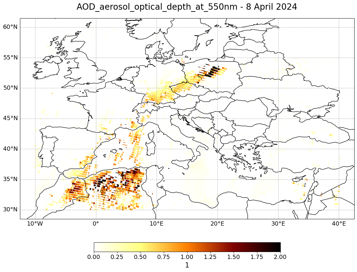
visualize_scatter(xr_dataarray=aod_xr_subset, 
                  conversion_factor=1, 
                  projection=ccrs.PlateCarree(),
                  vmin=0,
                  vmax=1, 
                  point_size=10,
                  color_scale='afmhot_r', 
                  unit=aod.Units, 
                  title=aod.Long_name + ' ' + '- 2021-02-06')

Dust Aerosol Detection, Monitoring and Forecasting

Polar Multi-Sensor Aerosol Optical Properties (PMAp) Product

Contents